Getting performance from the MD algorithm
Questions
What aspects of the MD algorithm are most important for performance?
What do I need to know as a user to understand the performance?
Objectives
Be able to name the most important parts of the MD workflow
Appreciate some of the internal architecture of mdrun
Workflow within an MD simulation

Stages of the iterative pipeline that is implemented by molecular dynamics engines like mdrun
How long it takes to compute a stage of the pipeline depends on two factors:
how fast the arithmetic needs to be done
how fast the data moves to where it needs to be
The latter gets harder when GPUs are involved, because they are physically separated from the CPU. Fortunately, they also tend to make the former possible to make faster. Unfortunately, which one dominates is hard to analyse in general. The amount of arithmetic varies for each simulation system, and how long it would take to move the data somewhere else to do the arithmetic isn’t known in advance. Diversity makes our lives hard, both as users and developers!
The good news is that most of the arithmetic is in the force calculation, so there is a natural place to focus effort.
How do GPUs help?
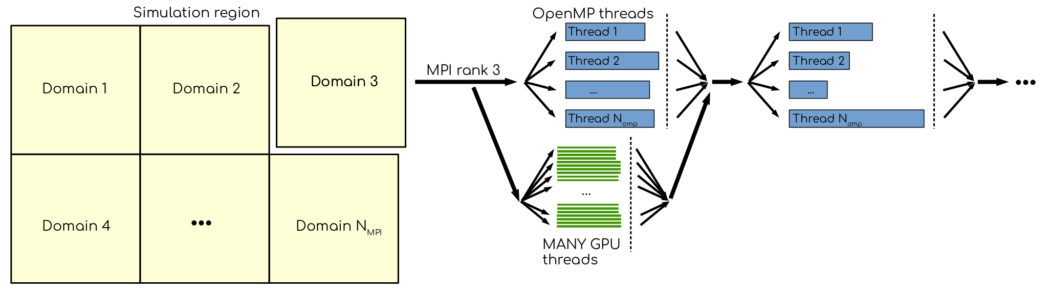
Using GPUs in addition to MPI ranks and OpenMP threads to explore parallelism. Many GPU threads can significantly speed-up the evaluation of compute-intense tasks. However, to get the best out of it, the domain has to contain thousands to tens of thousands off particles.
GPUs are electronic devices that are massively parallel, often with thousands of identical compute units ready to all do the same thing. This was developed for the challenge of rendering complex images onto computer screens, but the good work done there has also been built upon to do more general computation.
Before parallelism helps, we need to know that there is concurrency, ie that there are independent pieces of work that can be separated out. This is the same challenge we see in human teams… if Mary can’t start her work until Dinesh is done his piece, then those pieces of work are not concurrent. Hopefully, Mary has something else to do in the meantime until Dinesh is finished. But if not, the team is inefficient. Does MD have concurrency?
Fortunately, the forces we need to compute naturally come in a few classes, and those happen to be concurrent.

MD force fields use different components to describe different kinds of chemical interactions. Each has a set of static parameter data used to compute forces based on the positions. Those computations don’t depend on each other, so they are concurrent and may be parallelised.
Moving the most computationally intensive force-computation tasks to the GPU will let us exploit parallelism to compute faster.
2.1 Quiz: What is the best reason for moving the most computationally expensive tasks to the GPU?
CPUs cost more than GPUs
GPUs are good for computationally expensive tasks
They are the simplest to write GPU code for
It makes room for running many different kinds of tasks on the CPU in parallel with the GPU
Solution
Given that GROMACS already had a fast CPU implementation, moving the biggest workload to the GPU provides the best parallelism. There are grains of truth in the other answers, however.
Short-ranged non-bonded forces
For some kinds of system, it is enough to model the non-bonded forces by treating only short-ranged interactions. Because the Coulomb interaction between particles decays as \(\frac{1}{r}\) for distance \(r\), after a certain distance the interactions become neglible. Cancellation from similar contributions on the other side of a particle also helps here.
The simplest way to do this is to loop over all pairs of particles and compute the interactions only when \(r\) is within a pre-determined range. This works, but is highly inefficient, because the particles move slowly enough that it’s almost the same interacting set each time. Its cost also scales with the square of the number of particles \(N\), which is poor when \(N\) becomes large. So, instead a pair list is formed of particles that are close enough to interact (sometimes called a Verlet list or neighbor list). That pair list is re-used for many MD steps, until the diffusion of particles makes it necessary to rebuild it. It is also nice that this scales only with \(N\), too.

Molecular dynamics workflow for a system with only short-ranged non-bonded interactions.
Particles still diffuse across the boundary at each step, so GROMACS adds a buffer to the required interaction distance when building the list. At each step, the distance is checked when actually deciding whether to add the interaction to the forces. That is a source of inefficiency, but to do better we’d have to recompute the pair list more often, and that turns out to hurt more than helps! GROMACS will automatically determine a buffer size for you, based on your choice of an acceptable amount of drift in the total energy (see https://manual.gromacs.org/current/reference-manual/algorithms/molecular-dynamics.html#energy-drift-and-pair-list-buffering). The default values are quite defensive, but it is not recommended to change them because any performance benefit will be slight.
Further, it turns out that pair lists of single particles run slower than pair lists of clusters of particles. Small clusters of particles are normally either all interacting with each other, or all not interacting with each other, just like particles. Moving the data for the computation from memory to the compute unit is more efficient with small clusters, so GROMACS does it that way. The clusters have nothing to do with molecules or bonds, merely that the particles in them are close together. On GPUs, it turns out to be most efficient to group those clusters into clusters of clusters, also!
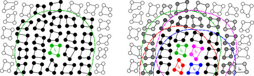
Illustration of clusters of four particles. Left panel: CPU-centric setup. All clusters with solid lines are included in the pair list of cluster i1 (green). Clusters with filled circles have interactions within the buffered cutoff (green dashed line) of at least one particle in i1, while particles in clusters intersected by the buffered cutoff that fall outside of it represent an extra implicit buffer. Right panel: hierarchical super-clusters on GPUs. Clusters i1–i4 (green, magenta, red, and blue) are grouped into a super-cluster. Dashed lines represent buffered cutoffs of each i-cluster. Clusters with any particle in any region will be included in the common pair list. Particles of j-clusters in the joint list are illustrated by discs filled in black to gray; black indicates clusters that interact with all four i-clusters, while lighter gray shading indicates that a cluster only interacts with 1–3 i-cluster(s), e.g., jm only with i4. Image used with permission from https://doi.org/10.1063/5.0018516.
Bonded forces
Many interesting systems feature particles that have chemical bonds that are not modelled well by non-bonded interactions. These require evaluating quite different mathematical functions from the non-bonded interactions, so they make sense to execute separately. These can also be evaluated on either the CPU or the GPU.

Workflow with short-ranged on the GPU and bonded on the CPU. This
is the default behavior in GROMACS, and can be selected with gmx
mdrun -nb gpu -bonded cpu.

Workflow with both short-ranged and bonded on the GPU. This can be
selected with gmx mdrun -nb gpu -bonded gpu.
Now there are two different ways we can run on the GPU. One exploits parallelism with the CPU, and one does not.
2.2 Quiz: When would it be most likely to benefit from moving bonded interactions to the GPU?
Few bonded interactions and relatively weak CPU
Few bonded interactions and relatively strong CPU
Many bonded interactions and relatively weak CPU
Many bonded interactions and relatively strong CPU
Solution
Running two tasks on the GPU adds overhead there, and that offsets any benefit from speeding up the bonded work by running it on the GPU. If the CPU is powerful enough to finish the bonded work before the GPU finishes the short-ranged work, then exploiting the CPU-GPU parallelism is best.
Explore performance with bonded interactions
Make a new folder for this exercise, e.g. mkdir
performance-with-bonded; cd performance-with-bonded.
Download the run input file prepared to do 50000
steps of a reaction-field simulation. We’ll use it to experiment
with task assignment.
Download the job submission script where you will see
several lines marked **FIXME**. Remove the **FIXME** to
achieve the goal stated in the comment before that line. You will
need to refer to the information above to achieve that. Save the
file and exit. Note that this script was designed to run on the
Puhti cluster. If you are not running on Puhti, then you will need
to make further changes to this file. Check the documentation for
how to submit jobs to your cluster!
Submit the script to the SLURM job manager with sbatch
script.sh. It will reply something like Submitted batch job
4565494 when it succeeded. The job manager will write terminal
output to a file named like slurm-4565494.out. It may take a
few minutes to start and a few more minutes to run.
While it is running, you can use tail -f slurm*out to watch the
output. When it says “Done” then the runs are finished. Use Ctrl-C
to exit the tail command that you ran.
The *.log files contain the performance (in ns/day) of each run
on the last line. Use tail *log to see the last chunk of each
log file. Examine the performance in ns/day for each trajectory.
Have a look through the log files and see what you can learn.
Solution
You can download a working version of the batch
submission script. Its diff from the original is file
--- /home/runner/work/gromacs-gpu-performance/gromacs-gpu-performance/content/exercises/performance-with-bonded/script.sh
+++ /home/runner/work/gromacs-gpu-performance/gromacs-gpu-performance/content/answers/performance-with-bonded/script.sh
@@ -12,16 +12,15 @@
 module load gromacs-env/2021-gpu
 export OMP_NUM_THREADS=$SLURM_CPUS_PER_TASK

-
 # Make sure we don't spend time writing useless output
 options="-nsteps 20000 -resetstep 19000 -ntomp $SLURM_CPUS_PER_TASK -pin on -pinstride 1"

 # Run mdrun with the default task assignment
 srun gmx mdrun $options -g default.log
 # Run mdrun assigning the non-bonded and bonded interactions to the GPU
-srun gmx mdrun $options -g manual-nb-bonded.log  **FIXME**
+srun gmx mdrun $options -g manual-nb-bonded.log  -nb gpu -bonded gpu
 # Run mdrun assigning only the non-bonded interactions to the GPU
-srun gmx mdrun $options -g manual-nb.log         **FIXME**
+srun gmx mdrun $options -g manual-nb.log         -nb gpu -bonded cpu

 # Let us know we're done
 echo Done
Sample output it produced is available:
The tails of those log files are
==> default.log <==

NOTE: 19 % of the run time was spent in pair search,
      you might want to increase nstlist (this has no effect on accuracy)

               Core t (s)   Wall t (s)        (%)
       Time:      326.182       16.310     1999.9
                 (ns/day)    (hour/ns)
Performance:      529.746        0.045
Finished mdrun on rank 0 Thu Sep  9 09:04:24 2021


==> manual-nb-bonded.log <==

NOTE: 18 % of the run time was spent in pair search,
      you might want to increase nstlist (this has no effect on accuracy)

               Core t (s)   Wall t (s)        (%)
       Time:      340.917       17.047     1999.9
                 (ns/day)    (hour/ns)
Performance:      506.852        0.047
Finished mdrun on rank 0 Thu Sep  9 09:04:44 2021


==> manual-nb.log <==

NOTE: 19 % of the run time was spent in pair search,
      you might want to increase nstlist (this has no effect on accuracy)

               Core t (s)   Wall t (s)        (%)
       Time:      322.644       16.133     1999.9
                 (ns/day)    (hour/ns)
Performance:      535.554        0.045
Finished mdrun on rank 0 Thu Sep  9 09:05:04 2021
Depending on the underlying variability of the performance of this trajectory on this hardware, we might be able to observe which configuration corresponds to the default, and whether offloading bonded interactions is advantageous, or not. Run the scripts a few times to get a crude impression of that variability!
Keypoints
Concurrent force calculations can be computed in parallel
GROMACS handles buffered short-range interactions automatically for you