Introduction to Julia syntax

Questions

• How do I run Julia?

• What does basic Julia syntax look like?

Instructor note

• 20 min teaching

• 20 min exercises

This episodes provides a condensed overview of Julia’s main syntax and features.

Video alternative

As an alternative to going through this page, learners can also watch this video which covers “a 300 page book on Julia in one hour”.

Coming from other languages

If you are coming from MATLAB, R, Python, C/C++ or Common Lisp, you should also have a look at this page which lists the respective differences in Julia.

Running Julia

We can write Julia code in various ways:

1. REPL (read-evaluate-print-loop). Start it by typing julia (or the full path of your Julia executable) on your command line. The REPL has four modes:

   • Julian mode - default mode where prompt starts with julia>. Here you enter Julia expressions and see output.

   • Type ? to go to Help mode where prompt starts with help?>. Julia will print help/documentation on anything you enter.

   • Type ; to go to Shell mode where prompt starts with shell>. You can type any shell commands as you would from terminal.

   • Type ] to go to Package mode where prompt starts with (@v1.5) pkg> (if you have Julia version 1.5). Here you can add packages with add, update packages with update etc. To see all options type ?.

   • To exit any non-Julian mode, hit Backspace key.

2. Jupyter: Jupyter notebooks are familiar to many Python and R users.

3. Pluto.jl: Pluto offers a similar notebook experience to Jupyter, but in contrast to Jupyter, Pluto understands global references between cells, and reactively re-evaluates cells affected by a code change.

4. Visual Studio Code (VSCode):

   • a full-fledged Integrated Development Environment which is very useful for larger codebases. Extensions are needed to activate Julia inside VSCode, see the official documentation for instructions.

5. A text editor like nano, emacs, vim, etc., followed by running your code with julia filename.jl.

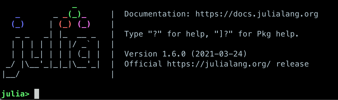
Firing up Julia

If Julia has been installed according to the instructions in Setup it should be possible to open up a Julia session by typing julia in a terminal window or by clicking on the Julia application in a file browser. The result should look something like this:

Basic syntax

Feature	Example syntax and its result/meaning
Arithmetic	2 + 3 * 1.1 Summing, multiplying 2^3 Power sqrt(9) Square root 40 / 5 8.0 (Float) 12 % 5 2 (remainder) 10^19 Results in integer overflow! 1e19 or big(10)^19 -> solves the problem exp(pi*im) Exponentiation, imaginary nr. sin(2*pi) Trigonometry
Types	A = 3.14 Scalar, float B = 10 Scalar, integer C = true Boolean D = 3+4im Complex E = "hello" String E[1] Char typeof(A) Find type supertype(Integer) Find supertypes subtypes(Integer) Find subtypes Integer <: Real “Subtype of”, returns True struct Immutable composite type mutable struct Mutable composite type :something Symbol for a name or label
Special values	Inf Infinity (e.g. 1 / 0) Nan Not a number (e.g. 0 / 0) nothing e.g. for variables w/o value

Let us explore some basic types in the Julia REPL:

typeof(1)
# Int64

typeof(1.0)
# Float64

typeof(1.0+2.0im)
# ComplexF64

supertypes(Float64)
# (Float64, AbstractFloat, Real, Number, Any)

subtypes(Real)
# 4-element Vector{Any}:
#  AbstractFloat
#  AbstractIrrational
#  Integer
#  Rational

Vectors and arrays

Feature	Example syntax and its result/meaning
1D arrays	t = (1, 2, 3) Tuple (immutable) t = (a=2, b=1+2) Named tuple, access: t.a d = Dict("A"=>1, "B"=>2) Dictionary a = [1, 2, 3, 4] 4-element Vector{Int64} a = [i^3 for i in [1,2,3]] Array comprehension Vector{T}(undef, n) undef 1-D array length n Float64[1,2] 2-element Vector{Float64} Array(1:5) 5-element Array{Int64,1} [1:5;] 5-element Array{Int64,1} [1:5] 1-element vector with a range [range(0,stop=2π,length=5);] 5-element Vector{Float64} collect(T, itr) array from iterable rand(5) random 5-elem vector in [0,1) rand(Int, 5) random vector with integers ones(5) 5-elem vector with FP64 ones zeros(5) 5-elem vector with FP64 zeros [1,2,3].^2 Element-wise operation
Indexing and slicing	a[1] first element a[1:3] 3-element vector a[3:end] end is last element a[1:2:end] step size of 2 a[3:end] end is last element splice!(a,2:3) Remove items at given indices splice!(a,2:3, 5:7) Rm & add items at given inds
Multidimensional arrays	Array{T}(undef, dims) New undef array type T mat = [1 2; 3 4] 2×2 Matrix{Int64} zeros(4,4,4,4) Zero 4×4×4×4 Array{Float64,4} rand(12,4) Random 12×4 Matrix{Float64}
Inspecting array properties	length(a) first(a) last(a) minimum(a) maximum(a) argmin(a) argmax(a) size(a)
Manipulating arrays	push!(a, 10) Append in-place insert!(a, 1, 42) Insert in given position append!(a, [3, 5, 7]) Append another array splice!(a, 3, -1) Rm in given pos and replace

We can play around with Vectors and Arrays to get used to their syntax:

v1 = [1.0, 2.0, 3.0]
# 3-element Vector{Int64}:
m1 = [1.0 2.0 3.0]
# 1×3 Matrix{Int64}:

# broadcasting
v2 = v1.^2
v3 = v2 .- v1

# slicing
v1[2:3]
v1[begin:2:end]

# combine vectors into matrix
A = [v1 v2 [7.0, 6.0, 5.0]]
size(A)
length(A)
A[1:2, 1] = [3,3] # types are cast automatically

# solve Ax=b
b = [4.0, 3.0, 2.0]
x = A \ b

# test with matrix-vector multiply
A*x == b
# true

Loops and conditionals

for loops iterate over iterables, including types like Range, Array, Set and Dict.

for i in [1,2,3,4,5]
    println("i = $i")
end

A = [1 2; 3 4]
# visit each index of A efficiently
for i in eachindex(A)
    println("i = $i, A[i] = $(A[i])")
end

for (k, v) in Dict("A" => 1, "B" => 2, "C" => 3)
    println("$k is $v")
end

for (i, j) in ([1, 2, 3], ("a", "b", "c"))
    println("$i $j")
end

Conditionals work like in other languages.

if x > 5
    println("x > 5")
elseif x < 5    # optional elseif
    println("x < 5")
else            # optional else
    println("x = 5")
end

The ternary operator exists in Julia:

a ? b : c

The meaning is [condition] ? [execute if true] : [execute if false].

While loops:

n = 0
while n < 10
    n += 1
    println(n)
end

Working with files

Obtain a file handle to start reading from file, and then close it:

f = open("myfile.txt")
# work with file...
close(f)

The recommended way to work with files is to use a do-block. At the end of the do-block the file will be closed automatically:

open("myfile.txt") do f
    # read from file
    lines = readlines(f)
    println(lines)
end

Writing to a file:

open("myfile.txt", "w") do f
    write(f, "another line")
end

Some useful functions to work with files:

Function	What it does
pwd()	Show current directory
cd(path)	Change directory
readdir(path)	Return list of current directory
mkdir(path)	Create directory
abspath(path)	Add current dir to filename
joinpath(p1, p2)	Join two paths
isdir(path)	Check if path is a directory
splitdir(path)	Split path into tuple of dirname and filename
homedir()	Return home directory

Functions

A function is an object that maps a tuple of argument values to a return value.

Example of a regular, named function:

function f(x,y)
    x + y   # can also use "return" keyword
end

A more compact form:

f(x,y) = x + y

This function can be called by f(4,5).

The expression f refers to the function object, and can be passed around like any other value (functions in Julia are first-class objects):

g = f
g(4,5)

Functions can be combined by composition:

f(x) = x^2
g(x) = sqrt(x)

f(g(3))   # returns 3.0

An alternative syntax is to use ∘ (typed by \circ<tab>)

(f ∘ g)(3)   # returns 3.0

Most operators (+, -, * etc) are in fact functions, and can be used as such:

+(1, 2, 3)   # 6

# composition:
(sqrt ∘ +)(3, 6)  # 3.0 (first summation, then square root)

Just like Vectors and Arrays can be operated on element-wise (vectorized) by dot-operators (e.g. [1, 2, 3].^2), functions can also be vectorized (broadcasting):

sin.([1.0, 2.0, 3.0])

Keyword arguments can be added after ;:

function greet_dog(; greeting = "Hi", dog_name = "Fido")  # note the ;
    println("$greeting $dog_name")
end

greet_dog(dog_name = "Coco", greeting = "Go fetch")   # "Go fetch Coco"

Optional arguments are given default value:

function date(y, m=1, d=1)
    month = lpad(m, 2, "0")  # lpad pads from the left
    day = lpad(d, 2, "0")
    println("$y-$month-$day")
end

date(2021)   # "2021-01-01
date(2021, 2)   # "2021-02-01
date(2021, 2, 3)   # "2021-02-03

Argument types can be specified explicitly:

function f(x::Float64, y::Float64)
    return x*y
end

Return types can also be specified:

function g(x, y)::Int8
    return x * y
end

Additional methods can be added to functions simply by new definitions with different argument types:

function f(x::Int64, y::Int64)
    return x*y
end

To find out which method is being dispatched for a particular function call:

@which f(3, 4)

As functions in Julia are first-class objects, they can be passed as arguments to other functions. Anonymous functions are useful for such constructs:

map(x -> x^2 + 2x - 1, [1, 3, -1])  # passes each element of the vector to the anonymous function

Varargs functions can take an arbitrary number of arguments:

f(a,b,x...) = a + b + sum(x)

f(1,2,3)     # 6
f(1,2,3,4)   # 10

“Splatting” is when values contained in an iterable collection are split into individual arguments of a function call:

x = (3, 4, 5)

f(1,2,x...)    # 15

# also possible:
x = [1, 2, 3, 4, 5]

f(x...)    # 15

Julia functions can be piped (chained) together:

1:10 |> sum |> sqrt    # 7.416198487095663 (first summed, then square root)

Inbuilt functions ending with ! mutate their input variables, and this convention should be adhered to when writing own functions. Compare, for example:

A = [1 2; 3 4]
sum(A)   # gives 10
sum!([1 1], A)  # mutates A into 1x2 Matrix with elements 4, 6

Exception handling

Exceptions are thrown when an unexpected condition has occurred:

sqrt(-1)

DomainError with -1.0:
sqrt will only return a complex result if called with a complex argument. Try sqrt(Complex(x)).

Stacktrace:
  [1] throw_complex_domainerror(::Symbol, ::Float64) at ./math.jl:33
  [2] sqrt at ./math.jl:573 [inlined]
  [3] sqrt(::Int64) at ./math.jl:599
  [4] top-level scope at In[130]:1
  [5] include_string(::Function, ::Module, ::String, ::String) at ./loading.jl:1091

Exceptions can be handled with a try/catch block:

try
    sqrt(-1)
catch e
    println("caught the error: $e")
end

caught the error: DomainError(-1.0, "sqrt will only return a complex result if called with a complex argument. Try sqrt(Complex(x)).")

Exceptions can be created explicitly with throw:

function negexp(x)
    if x>=0
        return exp(-x)
    else
        throw(DomainError(x, "argument must be non-negative"))
    end
end

The @assert macro can be used to throw an AssertionError if a condition does not hold:

@assert iseven(3) "3 is an odd number!"
# ERROR: AssertionError: 3 is an odd number!

Scope

The scope of a variable is the region of code within which a variable is visible. Certain constructs introduce scope blocks:

• Modules introduce a global scope that is separate from the global scopes of other modules.

• There is no all-encompassing global scope.

• Functions and macros define hard local scopes.

• for, while and try blocks and structs define soft local scopes.

When x = 123 occurs in a local scope, the following rules apply:

• Existing local: If x is already a local variable, then the existing local x is assigned.

• Hard scope: If x is not already a local variable, a new local named x is created in the same scope.

• Soft scope: If x is not already a local variable the behavior depends on whether the global variable x is defined:

  • if global x is undefined, a new local named x is created.

  • if global x is defined, the assignment is considered ambiguous.

Examples:

x = 123 # global

# hard scope
function greet()
    x = "hello" # new local
    println(x)
end

greet()  # gives "hello"
println(x)  # gives 123

function greet2()
    global x = "hello"
end

greet2()
println(x)  # gives "hello" (global x redefined)

# soft scope
x = 123
for i in 1:3
    x = i
end
println(x)
# returns 3

x = 123
for i in 1:3
    local x = i
end
println(x)
# returns 123

Further details can be found at https://docs.julialang.org/en/v1/manual/variables-and-scoping/

Style conventions

• Names of variables are in lower case.

• Word separation can be indicated by underscores (_), but use of underscores is discouraged unless the name would be hard to read otherwise.

• Names of Types and Modules begin with a capital letter and word separation is shown with upper camel case instead of underscores.

• Names of functions and macros are in lower case, without underscores.

• Functions that write to their arguments have names that end in !. These are sometimes called “mutating” or “in-place” functions because they are intended to produce changes in their arguments after the function is called, not just return a value.

Exercises

Practice yourself

Was anything unclear or covered too fast in the walkthrough above? Revisit it, read the material, play around yourself and ask questions in the shared workshop document!

Row vs column-major ordering?

Based on the output of the following loop:

A = [1 2; 3 4]
# visit each index of A efficiently
for i in eachindex(A)
    println("i = $i, A[i] = $(A[i])")
end

can you tell whether Julia is row or column-major ordered? (i.e., whether arrays are stacked one row or one column at a time in memory)

Solution

This code produces the following output:

# i = 1, A[i] = 1
# i = 2, A[i] = 3
# i = 3, A[i] = 2
# i = 4, A[i] = 4

which shows that Julia loops over columns since it’s a column-major language!

Reading files

Write a function which opens and reads a file and returns the number of words in it. Here are example codes for this task in other languages which you can translate:

PythonC++R

def count_word_occurrence_in_file(file_name, word):
    """
    Counts how often word appears in file file_name.
    Example: if file contains "one two one two three four"
             and word is "one", then this function returns 2
    """
    count = 0
    with open(file_name, 'r') as f:
        for line in f:
            words = line.split()
            count += words.count(word)
    return count

Solution

"""
    count_word_occurrence_in_file(file_name::String, word::String)

Counts how often word appears in file file_name.
Example: if file contains "one two one two three four"
         And word is "one", then this function returns 2
"""
function count_word_occurrence_in_file(file_name::String, word::String)
    open(file_name, "r") do file
        lines = readlines(file)
        return count(word, join(lines))
    end
end

FizzBuzz

Write a program that prints the integers from 1 to 100 (inclusive), except that:

• for multiples of three, print “Fizz” instead of the number

• for multiples of five, print “Buzz” instead of the number

• for multiples of both three and five, print “FizzBuzz” instead of the number

If you prefer translating a FizzBuzz code from your favorite language to Julia, you can find it on Rosetta Code.

Solution

for i in 1:100
    if i % 15 == 0
        println("FizzBuzz")
    elseif i % 3 == 0
        println("Fizz")
    elseif i % 5 == 0
        println("Buzz")
    else
        println(i)
    end
end

On the Rosetta Code page for FizzBuzz you find several other Julia versions.