Data Preparation using the Palmer Penguins Dataset

The Palmer Penguins Dataset is a popular dataset used in data science and machine learning education. The data was gathered between 2007 and 2009 by Dr. Kristen Gorman as part of the Palmer Station Long Term Ecological Research (LTER) Program. It contains measurements for 344 penguins from three species – Adelie, Chinstrap, and Gentoo – collected from three islands (Biscoe, Dream, and Torgersen) in the Palmer Archipelago, Antarctica.

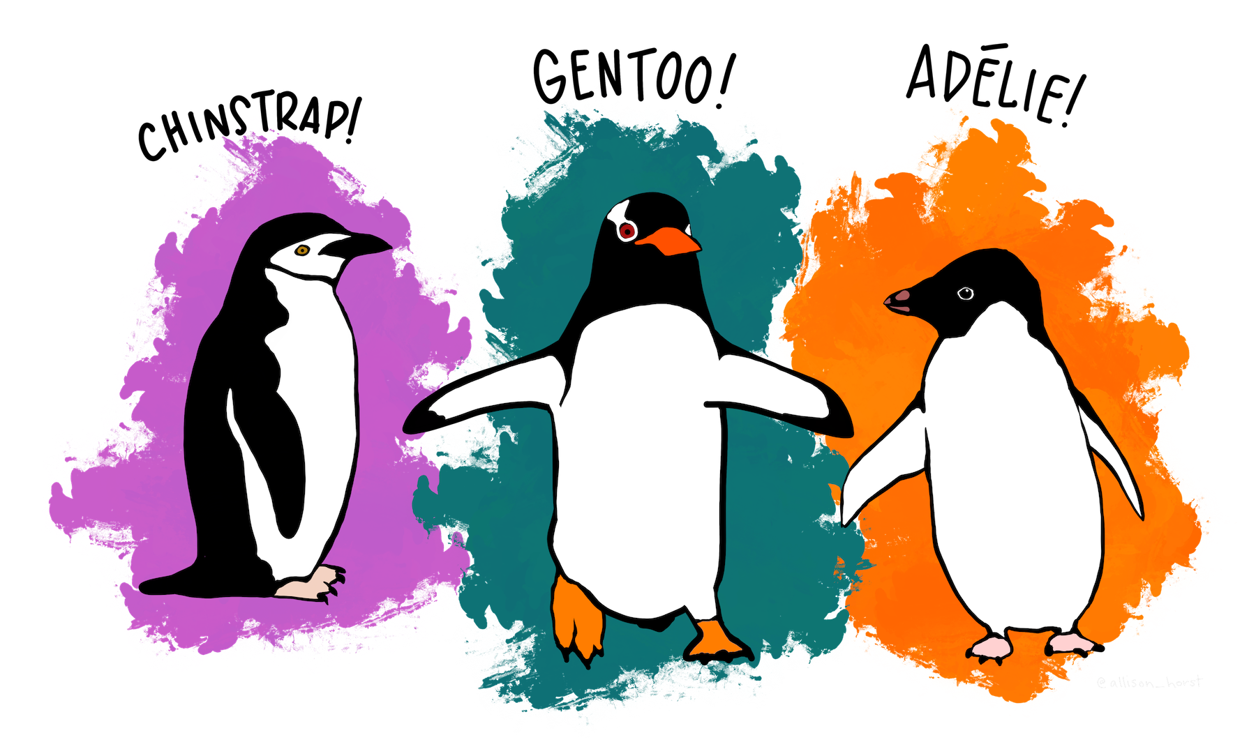
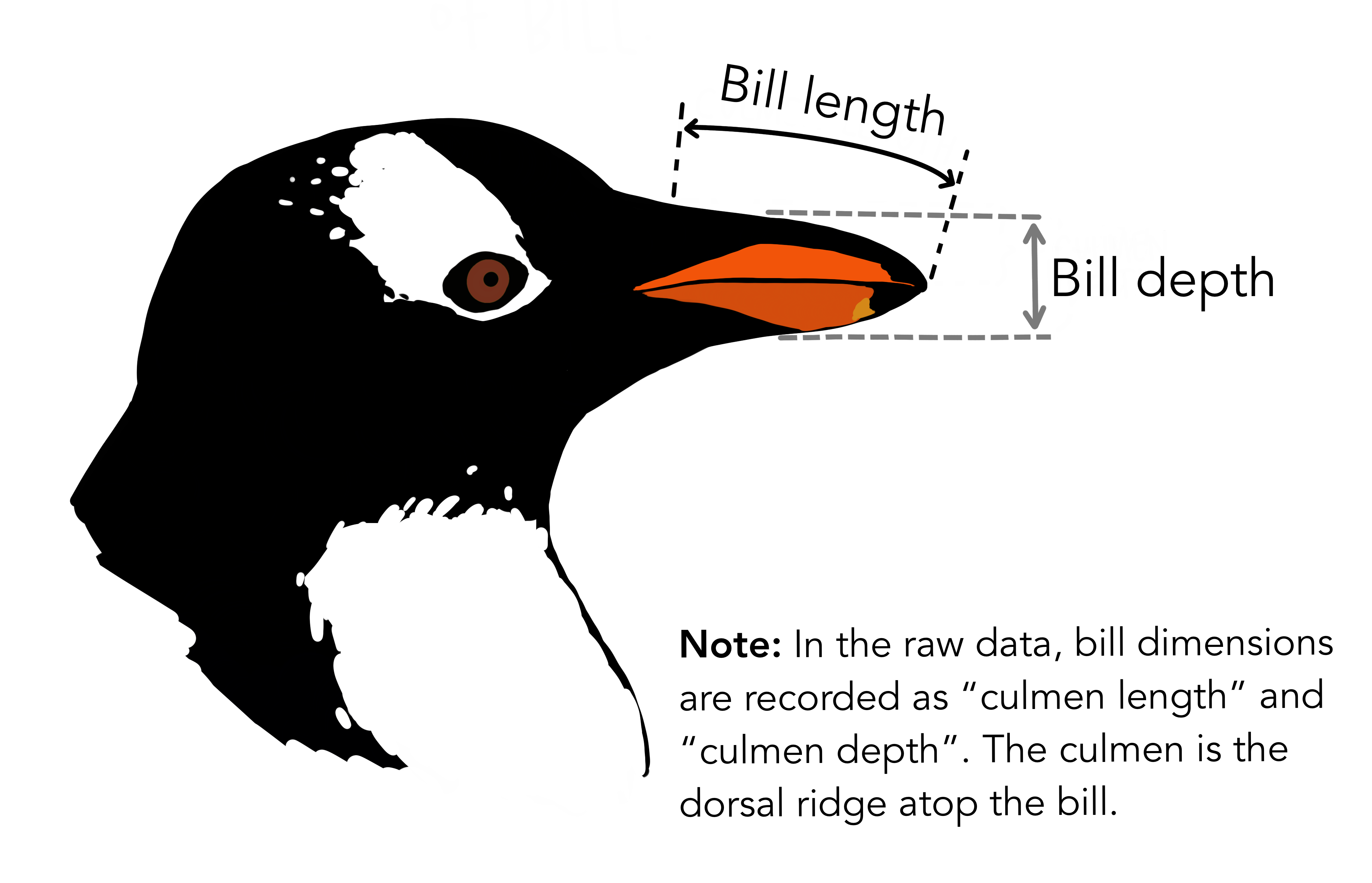
The physical attributes measured for penguins are flipper length, beak length, beak width, body mass, and sex.

1. Loading Dataset

import numpy as np
import pandas as pd
import matplotlib.pyplot as plt
import seaborn as sns

# penguins = pd.read_csv("./penguins_dataset.csv")

# URL of the Penguins dataset (CSV file)
# url = "https://raw.githubusercontent.com/mwaskom/seaborn-data/master/penguins.csv"
# penguins = pd.read_csv(url)

penguins = sns.load_dataset('penguins')
penguins

penguins.info()

penguins.describe()

sns.pairplot(penguins, hue="sex", height=2.0)

sns.pairplot(penguins, hue="island", height=2.0)

sns.pairplot(penguins[["species", "bill_length_mm", "bill_depth_mm", "flipper_length_mm", "body_mass_g"]], hue="species", height=2.0)

2. Handling Missing Values

penguins_test = pd.concat([penguins.head(5), penguins.tail(5)])
penguins_test.style.highlight_null(color = 'red')

2.1 Handling missing numerical data

Mean or Median Imputation

# calculate `mean` and `median` of body_mass data

body_mass_g_mean = penguins_test.body_mass_g.mean()
body_mass_g_median = penguins_test.body_mass_g.median()
print(f"  mean value of body_mass_g is {body_mass_g_mean}")
print(f"median value of body_mass_g is {body_mass_g_median}")

penguins_test['BMG_mean'] = penguins_test.body_mass_g.fillna(body_mass_g_mean)
penguins_test['BMG_median'] = penguins_test.body_mass_g.fillna(body_mass_g_median)
penguins_test.style.highlight_null(color = 'green')

plt.figure(figsize=(8, 6))

penguins_test['body_mass_g'].plot(kind='kde', color='tab:green', label="body_mass_g")
penguins_test['BMG_mean'].plot(kind='kde', color='tab:orange', label="BMG_mean")
penguins_test['BMG_median'].plot(kind='kde', color='tab:blue', label="BMG_median")

plt.legend(loc='best')
plt.tight_layout()

End of Distribution Imputation

Sometimes one would want to replace missing data with values at the tail of distribution of variable.
Advantage is that it is quick and captures importance of missing values (if one suspects missing data is valuable).
EoD’s extreme value means the mean value with 3rd stander deviation, (mean + (3*std)))

eod_value = penguins_test['body_mass_g'].mean() + 3 * penguins_test['body_mass_g'].std()
eod_value

penguins_test['BMG_eod'] = penguins_test.body_mass_g.fillna(eod_value)
penguins_test.style.highlight_null(color = 'green')

plt.figure(figsize=(8, 6))

penguins_test['body_mass_g'].plot(kind='kde', color='tab:green', label="body_mass_g")
penguins_test['BMG_mean'].plot(kind='kde', color='tab:orange', label="BMG_mean")
penguins_test['BMG_median'].plot(kind='kde', color='tab:blue', label="BMG_median")
penguins_test['BMG_eod'].plot(kind='kde', color='tab:red', label="BMG_eod")

plt.legend(loc='best')
plt.tight_layout()

2.2 Handling missing categorical data

penguins_test.style.highlight_null(color = 'red')

# Frequent Category Imputation (mode imputation): replace missing values with the most frequent category

plt.figure(figsize=(8, 6))

penguins_test.sex.value_counts().sort_values(ascending=False).plot.bar()

plt.xlabel('Sex')
plt.ylabel('Number of Penguins')

plt.tight_layout()

print("mode for sex feature: \n", penguins_test.sex.mode())

print("Before mode imputation: \n", penguins_test['sex'], '\n')

penguins_test_sex_mode = penguins_test['sex'].fillna(penguins_test.sex.mode()[0])
print("After mode imputation: \n", penguins_test_sex_mode)

plt.figure(figsize=(8, 6))

dataset = []
female = []
male = []

dataset.append("Raw data")
female.append(penguins_test.sex.value_counts()["Female"])
male.append(penguins_test.sex.value_counts()["Male"])

dataset.append("Frequent Category Imputation")
female.append(penguins_test_sex_mode.value_counts()["Female"])
male.append(penguins_test_sex_mode.value_counts()["Male"])

x_axis = np.arange(len(dataset))

plt.bar(x_axis - 0.2, female, width=0.4, label = 'Female')
plt.bar(x_axis + 0.2, male, width=0.4, label = 'Male')

# plt.xticks(x_axis, team)

plt.xlabel('Sex')
plt.ylabel('Number of Penguins')

plt.tight_layout()
plt.legend()

Constant Value Imputation

# Constant Value Imputation

penguins_test_sex_missing = penguins_test['sex'].fillna("Missing")
print(penguins_test_sex_missing)

plt.figure(figsize=(8, 6))

penguins_test_sex_missing.value_counts().sort_values(ascending=False).plot.bar()

plt.xlabel('Sex')
plt.ylabel('Number of Penguins')

plt.tight_layout()

2.3 Remove missing values

penguins_test.style.highlight_null(color = 'red')

penguins_test_remove = penguins_test.dropna() # axis=1
penguins_test_remove.style.highlight_null(color = 'red')

3. Handling Outliers

eod_value = penguins['body_mass_g'].mean() + 3 * penguins_test['body_mass_g'].std()
print(f"EoD value = {eod_value}")

penguins_test_BMG_outlier = penguins[["species", "bill_length_mm", "body_mass_g"]]

penguins_test_BMG_outlier.loc[:, "body_mass_g"] = penguins_test_BMG_outlier["body_mass_g"].fillna(eod_value)
penguins_test_BMG_outlier

3.1 How to define outlier?

plt.figure(figsize=(8, 6))

sns.swarmplot(y=penguins_test_BMG_outlier["species"], x=penguins_test_BMG_outlier["body_mass_g"],
              color="lightgreen", marker="o", size=4)

sns.boxplot(y=penguins_test_BMG_outlier["species"], x=penguins_test_BMG_outlier["body_mass_g"], 
            palette="coolwarm", notch=True, linewidth=2, width=0.5, 
            hue=penguins_test_BMG_outlier.species, legend=False)

plt.xlabel("Body mass (g)", fontsize=14)
plt.ylabel("Species", fontsize=14)
plt.tick_params(axis='x', labelsize=12)
plt.tick_params(axis='y', labelsize=12)

plt.tight_layout()

3.2 The Inter quartile range (IQR) method

penguins_test_BMG_outlier.describe()

print(f"25% quantile = {penguins_test_BMG_outlier['body_mass_g'].quantile(0.25)}")
print(f"75% quantile = {penguins_test_BMG_outlier['body_mass_g'].quantile(0.75)}\n")

IQR = penguins_test_BMG_outlier["body_mass_g"].quantile(0.75) - penguins_test_BMG_outlier["body_mass_g"].quantile(0.25)
lower_bmg_limit = penguins_test_BMG_outlier["body_mass_g"].quantile(0.25) - (1.5 * IQR)
upper_bmg_limit = penguins_test_BMG_outlier["body_mass_g"].quantile(0.75) + (1.5 * IQR)

print(f"lower limt of IQR = {lower_bmg_limit} and upper limit of IQR = {upper_bmg_limit}")

penguins_test_BMG_outlier[penguins_test_BMG_outlier["body_mass_g"] > upper_bmg_limit]

penguins_test_BMG_outlier[penguins_test_BMG_outlier["body_mass_g"] < lower_bmg_limit]

penguins_test_BMG_outlier_remove_IQR = penguins_test_BMG_outlier[penguins_test_BMG_outlier["body_mass_g"] < upper_bmg_limit]
penguins_test_BMG_outlier_remove_IQR

plt.figure(figsize=(8, 6))

sns.swarmplot(y=penguins_test_BMG_outlier_remove_IQR["species"], x=penguins_test_BMG_outlier_remove_IQR["body_mass_g"], color="lightgreen", marker="o", size=4)

sns.boxplot(y=penguins_test_BMG_outlier_remove_IQR["species"], x=penguins_test_BMG_outlier_remove_IQR["body_mass_g"], 
            palette="coolwarm", notch=True, linewidth=2, width=0.5, 
            hue=penguins_test_BMG_outlier_remove_IQR.species, legend=False)

plt.tight_layout()

3.3 The mean-standard deviation method

eod_value = penguins['body_mass_g'].mean() + 3 * penguins_test['body_mass_g'].std()
print(f"EoD value = {eod_value}")

penguins_test_BMG_outlier = penguins[["species", "bill_length_mm", "body_mass_g"]]

penguins_test_BMG_outlier.loc[:, "body_mass_g"] = penguins_test_BMG_outlier["body_mass_g"].fillna(eod_value)
penguins_test_BMG_outlier

mean = penguins_test_BMG_outlier["body_mass_g"].mean()
std = penguins_test_BMG_outlier["body_mass_g"].std()
print(f"mean = {mean}, std = {std}", '\n')

lower_bmg_limit = mean - (3.0 * std)
upper_bmg_limit = mean + (3.0 * std)

print(f"lower limt of mean-std = {lower_bmg_limit} and upper limit of mean-std = {upper_bmg_limit}")
# lower limt of IQR = 1703.125 and upper limit of IQR = 6628.125

penguins_test_BMG_outlier[penguins_test_BMG_outlier["body_mass_g"] > upper_bmg_limit]

penguins_test_BMG_outlier[penguins_test_BMG_outlier["body_mass_g"] < lower_bmg_limit]

test = penguins_test_BMG_outlier

penguins_test_BMG_outlier.loc[penguins_test_BMG_outlier["body_mass_g"] < lower_bmg_limit, "body_mass_g"] = mean
penguins_test_BMG_outlier.loc[penguins_test_BMG_outlier["body_mass_g"] > upper_bmg_limit, "body_mass_g"] = mean
penguins_test_BMG_outlier

4. Encoding Categorical Variables

penguins_sex = penguins[["species", "island", "sex"]].head(10)
penguins_sex

4.1 One hot encoding (OHE)

from sklearn.preprocessing import OneHotEncoder

encoder = OneHotEncoder(sparse_output=False)  # `sparse_output=False` to get a dense array
encoded = encoder.fit_transform(penguins_sex[['sex']])

encoded = pd.DataFrame(encoded, columns=["Female", "Male", "NaN"])

penguins_sex_onehotencoding = pd.concat([penguins_sex, encoded], axis=1)
penguins_sex_onehotencoding

4.2 Label encoding

penguins_sex

from sklearn.preprocessing import LabelEncoder

encoder = LabelEncoder()
encoded = encoder.fit_transform(penguins_sex['sex'])
encoded = pd.DataFrame(encoded, columns=["sex_LE"])

penguins_sex_labelencoding = pd.concat([penguins_sex, encoded], axis=1)
penguins_sex_labelencoding

4.3 The get_dummies() function in Pandas

penguins_sex

dummy_encoded = pd.get_dummies(penguins_sex['sex']).astype(np.int8)
penguins_sex_dummyencoding = pd.concat([penguins_sex, dummy_encoded], axis=1)
penguins_sex_dummyencoding