Intoduction to Horovod

Why Horovod

Horovod was developed at Uber with the primary motivation of making it easy to take a single-GPU training script and successfully scale it to train across many GPUs in parallel. This has two aspects:

How much modification does one have to make to a program to make it distributed, and how easy is it to run it?
How much faster would it run in distributed mode?

What researchers at Uber discovered was that the MPI model to be much more straightforward and require far less code changes than previous solutions such as Distributed TensorFlow with parameter servers. Once a training script has been written for scale with Horovod, it can run on a single-GPU, multiple-GPUs, or even multiple hosts without any further code changes.

In addition to being easy to use, Horovod is fast. Below is a chart representing the benchmark that was done on 128 servers with 4 Pascal GPUs each connected by RoCE-capable 25 Gbit/s network:

Horovod achieves 90% scaling efficiency for both Inception V3 and ResNet-101, and 68% scaling efficiency for VGG-16. While installing MPI and NCCL itself may seem like an extra hassle, it only needs to be done once by the team dealing with infrastructure, while everyone else in the company who builds the models can enjoy the simplicity of training them at scale. Plus, in modern clusters where GPUs are available, MPI and NCCL are readily installed. Installation of Horovod is not as difficult.

Main concept

Horovod core principles are based on the MPI concepts size, rank, local rank, allreduce, allgather, broadcast, and alltoall. These are best explained by example. Say we launched a training script on 4 servers, each having 4 GPUs. If we launched one copy of the script per GPU:

Size would be the number of processes, in this case, 16.
Rank would be the unique process ID from 0 to 15 (size - 1).
Local rank would be the unique process ID within the server from 0 to 3.
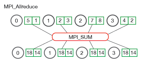
Allreduce is an operation that aggregates data among multiple processes and distributes results back to them. Allreduce is used to average dense tensors.
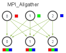
Allgather is an operation that gathers data from all processes on every process. Allgather is used to collect values of sparse tensors.
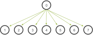
Broadcast is an operation that broadcasts data from one process, identified by root rank, onto every other process.
Alltoall is an operation to exchange data between all processes. Alltoall may be useful to implement neural networks with advanced architectures that span multiple devices.

How to use Horovod

To use Horovod, we should add the following to the program:

Run hvd.init() to initialize Horovod.

2. Pin each GPU to a single process to avoid resource contention. With the typical setup of one GPU per process, set this to local rank. The first process on the server will be allocated the first GPU, the second process will be allocated the second GPU, and so forth.

3. Scale the learning rate by the number of workers. Effective batch size in synchronous distributed training is scaled by the number of workers. An increase in learning rate compensates for the increased batch size.

4. Wrap the optimizer in hvd.DistributedOptimizer. The distributed optimizer delegates gradient computation to the original optimizer, averages gradients using allreduce or allgather, and then applies those averaged gradients.

5. Broadcast the initial variable states from rank 0 to all other processes. This is necessary to ensure consistent initialization of all workers when training is started with random weights or restored from a checkpoint.

6. Modify your code to save checkpoints only on worker 0 to prevent other workers from corrupting them.

Once the script is transformed to a proper form, it can be launched using horovodrun command. For example, to run the train scrip on a machine with 4 GPUs, we use

$ horovodrun -np 4 -H localhost:4 python train.py

And for running on 4 machines with 4 GPUs each, we use

horovodrun -np 16 -H server1:4,server2:4,server3:4,server4:4 python train.py

It is also possible to run the script using Open MPI without the horovodrun wrapper. The launch command for the first example using mpirun would be

mpirun -np 4 \
  -bind-to none -map-by slot \
  -x NCCL_DEBUG=INFO -x LD_LIBRARY_PATH -x PATH \
  -mca pml ob1 -mca btl ^openib \
  python train.py

And for the second example

mpirun -np 16 \
  -H server1:4,server2:4,server3:4,server4:4 \
  -bind-to none -map-by slot \
  -x NCCL_DEBUG=INFO -x LD_LIBRARY_PATH -x PATH \
  -mca pml ob1 -mca btl ^openib \
  python train.py

The recipe for running inside Jupyter Notebook is different, as we will see in the next section.

Training with `Model.fit`

Let’s go back to our CNN model for classification and upscale the training using Horovod.

There are three Horovod callbacks.

1. Horovod.broadcasts sends initial variable states from rank 0 to all other processes. This is necessary to ensure consistent initialization of all workers when training is started with random weights or restored from a checkpoint.

2. Horovod.metric.averages calculates metrics among workers at the end of every epoch. Note: This callback must be in the list before the ReduceLROnPlateau, TensorBoard or other metrics-based callbacks.

3. Horovod.LearningRateWarmup initializes the learning rate from the very beginning. Starting the training using `lr = 1.0 * hvd.size() with leads to worse final accuracy. This funciton scales the learning rate lr = 1.0 —> lr = 1.0 * hvd.size() during the first three epochs. See this article for details.

import horovod

def training_func():

  import tensorflow as tf
  import horovod.tensorflow as hvd

  hvd.init()

  # Pinning GPUs (one GPU per process)
  gpus = tf.config.experimental.list_physical_devices('GPU')
  for gpu in gpus:
      tf.config.experimental.set_memory_growth(gpu, True)
  if gpus:
      tf.config.experimental.set_visible_devices(gpus[hvd.local_rank()], 'GPU')

  (mnist_images, mnist_labels), _ = tf.keras.datasets.mnist.load_data(path='mnist-%d.npz' % hvd.rank())

  dataset = tf.data.Dataset.from_tensor_slices(
      (tf.cast(mnist_images[..., tf.newaxis] / 255.0, tf.float32),
       tf.cast(mnist_labels, tf.int64)))
  batch_size = 128
  dataset = dataset.repeat().shuffle(10000).batch(batch_size)

  # Horovod: adjust learning rate based on number of GPUs.
  scaled_lr = 0.001 * hvd.size()
  opt = tf.optimizers.Adam(scaled_lr)
  opt = hvd.DistributedOptimizer(opt, backward_passes_per_step=1, average_aggregated_gradients=True)

  mnist_model = tf.keras.Sequential([
      tf.keras.layers.Conv2D(32, 3, activation='relu'),
      tf.keras.layers.MaxPooling2D(),
      tf.keras.layers.Conv2D(64, 3, activation='relu'),
      tf.keras.layers.MaxPooling2D(),
      tf.keras.layers.Flatten(),
      tf.keras.layers.Dense(64, activation='relu'),
      tf.keras.layers.Dense(10, activation='softmax')
  ])

  mnist_model.compile(loss=tf.losses.SparseCategoricalCrossentropy(),
                  optimizer=opt,
                  metrics=['accuracy'],
                  experimental_run_tf_function=False)

  callbacks = [
  horovod.tensorflow.keras.callbacks.BroadcastGlobalVariablesCallback(0),
  horovod.tensorflow.keras.callbacks.MetricAverageCallback(),
  horovod.tensorflow.keras.callbacks.LearningRateWarmupCallback(initial_lr=scaled_lr,
  warmup_epochs=3, verbose=1),
  ]

  if hvd.rank() == 0:
      callbacks.append(tf.keras.callbacks.ModelCheckpoint('./checkpoint-{epoch}.h5'))

  verbose = 1 if hvd.rank() == 0 else 0

  mnist_model.fit(dataset, steps_per_epoch=500 // hvd.size(), callbacks=callbacks, epochs=24, verbose=verbose)

To launch the training, we need to use this command in the Jupyter notebook

horovod.run(training_func, np=2, verbose=False, disable_cache=True, use_mpi=True)

verbose = True

Change the verbose variable to True and inspect the results. What do you see?
Time the calculations. Can you compare the result with the results reported in Distributed training in TensorFlow?

Playing with Horovod

1. Play with different parameters in the code and check the effect on the elapsed time and accuracy. which parameters are more important?

2. Use Horovod using Keras Model.fit, similar to the above, to upscale SVHN notebook you worked before. Are the results comparable to those in the section Distributed training in TensorFlow?

Instead of using Model.fit, write a custom training loop within the framework of Horovod.

Solution

Two main differences that should be made are:

Definig the loss function using Horovod

@tf.function
def training_step(images, labels, first_batch):
    with tf.GradientTape() as tape:
          probs = mnist_model(images, training=True)
          loss_value = loss(labels, probs)

    # Horovod: add Horovod Distributed GradientTape.
    tape = hvd.DistributedGradientTape(tape)

    grads = tape.gradient(loss_value, mnist_model.trainable_variables)
    opt.apply_gradients(zip(grads, mnist_model.trainable_variables))

    # Horovod: broadcast initial variable states from rank 0 to all other processes.
    # This is necessary to ensure consistent initialization of all workers when
    # training is started with random weights or restored from a checkpoint.
    # Please see `the documentation <https://horovod.readthedocs.io/en/stable/api.html#horovod.tensorflow.broadcast_variables>`_.
    # Note: broadcast should be done after the first gradient step to ensure optimizer
    # initialization.

    if first_batch:
        hvd.broadcast_variables(mnist_model.variables, root_rank=0)
        hvd.broadcast_variables(opt.variables(), root_rank=0)

    return loss_value

Looping over the dataset

for batch, (images, labels) in enumerate(dataset.take(10000 // hvd.size())):
    loss_value = training_step(images, labels, batch == 0)

    if batch % 10 == 0 and hvd.local_rank() == 0:
        print('Step #%d\tLoss: %.6f' % (batch, loss_value))

It is possible to carry the same procedure without using Jupyter notebook as the main developing tool. You can download the python script from the github. We will go through some of the steps together.