Intoduction to Horovod

(Image Source)

Why Horovod

Horovod was developed at Uber with the primary motivation of making it easy to take a single-GPU training script and successfully scale it to train across many GPUs in parallel. This has two aspects:

• How much modification does one have to make to a program to make it distributed, and how easy is it to run it?

• How much faster would it run in distributed mode?

What researchers at Uber discovered was that the MPI model to be much more straightforward and require far less code changes than previous solutions such as Distributed TensorFlow with parameter servers. Once a training script has been written for scale with Horovod, it can run on a single-GPU, multiple-GPUs, or even multiple hosts without any further code changes.

In addition to being easy to use, Horovod is fast. Below is a chart representing the benchmark that was done on 128 servers with 4 Pascal GPUs each connected by RoCE-capable 25 Gbit/s network:

Horovod achieves 90% scaling efficiency for both Inception V3 and ResNet-101, and 68% scaling efficiency for VGG-16. While installing MPI and NCCL itself may seem like an extra hassle, it only needs to be done once by the team dealing with infrastructure, while everyone else in the company who builds the models can enjoy the simplicity of training them at scale. Plus, in modern clusters where GPUs are available, MPI and NCCL are readily installed. Installation of Horovod is not as difficult.

Alex Sergeev and Mike Del Balso, the researchers behind the development of Horovod at Uber, published an excellent history and review of the Hovorod. Here are some points they mentioned in their article:

• The first try for distributed training was based on TensorFlow distributed method. However, they experienced two major difficulties: 1. Difficulty of following instructions given by TensorFlow. In particular, they found the newly introduced concepts by TensorFlow for distributed training causes hard-to-diagnose bugs that slowed training.

• The second issue dealt with the challenge of computing at Uber’s scale. After running a few benchmarks, they found that they could not get the standard distributed TensorFlow to scale as well as our services required. For example, about half of their resources was lost due to scaling inefficiencies when training on 128 GPUs.

• An article by Facebook researchers entitled “Accurate, Large Minibatch SGD: Training ImageNet in 1 Hour, demonstrating their training of a ResNet-50 network in one hour on 256 GPUs by combining principles of data parallelism peaked their interests.

• A paper published by Baidu researchers in early 2017, “Bringing HPC Techniques to Deep Learning,” evangelizing a different algorithm for averaging gradients and communicating those gradients to all nodes, called ring-allreduce. The algorithm was based on the approach introduced in the 2009 paper “Bandwidth Optimal All-reduce Algorithms for Clusters of Workstations” by Patarasuk and Yuan.

(Image Source)

• The realization that a ring-allreduce approach can improve both usability and performance motivated them to work on our own implementation to address Uber’s TensorFlow needs.

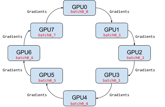
• Horovod (Khorovod) is named after a traditional Russian folk dance in which performers dance with linked arms in a circle, much like how distributed TensorFlow processes use Horovod to communicate with each other.

(Image Source)

• They replaced the Baidu ring-allreduce implementation with NCCL. NCCL provides a highly optimized version of ring-allreduce. NCCL 2 introduced the ability to run ring-allreduce across multiple machines, enabling us to take advantage of its many performance boosting optimizations.

Main concept

Horovod’s connection to MPI is deep, and for those familiar with MPI programming, much of what you program to distribute model training with Horovod will feel familiar.

Four core principles that Horovod is based on are the MPI concepts: size, rank, local rank, allreduce, allgather, broadcast, and alltoall. These are best explained by example. Say we launched a training script on 4 servers, each having 4 GPUs. If we launched one copy of the script per GPU:

• Size would be the number of processes, in this case, 16.

• Rank would be the unique process ID from 0 to 15 (size - 1).

• Local rank would be the unique process ID within the server from 0 to 3.

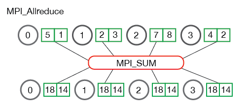
• Allreduce is an operation that aggregates data among multiple processes and distributes results back to them. Allreduce is used to average dense tensors.

  

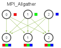
• Allgather is an operation that gathers data from all processes on every process. Allgather is used to collect values of sparse tensors.

  

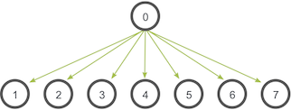
• Broadcast is an operation that broadcasts data from one process, identified by root rank, onto every other process.

  

• Alltoall is an operation to exchange data between all processes. Alltoall may be useful to implement neural networks with advanced architectures that span multiple devices.

(Images Source)

Horovod, as with MPI, strictly follows the Single-Program Multiple-Data (SPMD) paradigm where we implement the instruction flow of multiple processes in the same file/program. Because multiple processes are executing code in parallel, we have to take care about race conditions and also the synchronization of participating processes.

Horovod assigns a unique numerical ID or rank (an MPI concept) to each process executing the program. This rank can be accessed programmatically. As you will see below when writing Horovod code, by identifying a process’s rank programmatically in the code we can take steps such as:

• Pin that process to its own exclusive GPU.

• Utilize a single rank for broadcasting values that need to be used uniformly by all ranks.

• Utilize a single rank for collecting and/or reducing values produced by all ranks.

• Utilize a single rank for logging or writing to disk.

How to use Horovod

To use Horovod, we should add the following to the program:

1. Use hvd.init() to initialize Horovod.

2. Pin each GPU to a single process. This is to avoid resource contention. With the typical setup of one GPU per process, set this to local rank. The first process on the server will be allocated the first GPU, the second process will be allocated the second GPU, and so forth.

# Horovod: pin GPU to be used to process local rank (one GPU per process)
gpus = tf.config.experimental.list_physical_devices('GPU')
for gpu in gpus:
    tf.config.experimental.set_memory_growth(gpu, True)
if gpus:
    tf.config.experimental.set_visible_devices(gpus[hvd.local_rank()], 'GPU')

3. Print Verbose Logs Only on the First Worker. When running on several N processors, all N TensorFlow processes printed their progress to stdout (standard output). We only want to see the state of the output once at any given time. To accomplish this, we can arbitrarily select a single rank to display the training progress. By convention, we typically call rank 0 the “root” rank and use it for logistical work such as I/O when only one rank is required.

4. Add Distributed Optimizer. In the previous two sections we ran with multiple processes, but each process was running completely independently – this is not data parallel training, it is just multiple processes running serial training at the same time. The key step to make the training data parallel is to average out gradients across all workers, so that all workers are updating with the same gradients and thus moving in the same direction. Horovod implements an operation that averages gradients across workers. Deploying this in your code is very straightforward and just requires wrapping an existing optimizer (keras.optimizers.Optimizer) with a Horovod distributed optimizer (horovod.keras.DistributedOptimizer).

5. Initialize Random Weights on Only One Processor. Data parallel stochastic gradient descent, at least in its traditionally defined sequential algorithm, requires weights to be synchronized between all processors. We already know that this is accomplished for backpropagation by averaging out the gradients among all processors prior to the weight updates. Then the only other required step is for the weights to be synchronized initially. Assuming we start from the beginning of the training (we’ll handle checkpoint/restart later), this means that every processor needs to have the same random weights. In a previous section, we mentioned that the first worker would broadcast parameters to the rest of the workers. We will use horovod.keras.callbacks.BroadcastGlobalVariablesCallback to make this happen.

6. Modify Training Loop to Execute Fewer Steps Per Epoch. As it stands, we are running the same number of steps per epoch for the serial training implementation. But since we have increased the number of workers by a factor of N, that means we’re doing N times more work (when we sum the amount of work done over all processes). Our target was to get the same answer in less time (that is, to speed up the training), so we want to keep the total amount of work done the same (that is, to process the same number of examples in the dataset). This means we need to do a factor of N fewer steps per epoch, so the number of steps goes to steps_per_epoch / number_of_workers. We will also speed up validation by validating 3 * num_test_iterations / number_of_workers steps on each worker. While we could just do num_test_iterations / number_of_workers on each worker to get a linear speedup in the validation, the multiplier 3 provides over-sampling of the validation data and helps to increase the probability that every validation example will be evaluated.

7. Average Validation Results Among Workers. Since we are not validating the full dataset on each worker anymore, each worker will have different validation results. To improve validation metric quality and reduce variance, we will average validation results among all workers. To do so, we can use horovod.keras.callbacks.MetricAverageCallback.

8. Do Checkpointing Logic Only Using the Root Worker. The most important issue is that there can be a race condition while writing the checkpoint to a file. If every rank finishes the epoch at the same time, they might be writing to the same filename, and this could result in corrupted data. But more to the point, we don’t even need to do this: by construction in synchronous data parallel SGD, every rank has the same copy of the weights at all times, so only one worker needs to write the checkpoint. As usual, our convention will be that the root worker (rank 0) handles this.

9. Increase the learning rate. Given a fixed batch size per GPU, the effective batch size for training increases when you use more GPUs, since we average out the gradients among all processors. Standard practice is to scale the learning rate by the same factor that you have scaled the batch size – that is, by the number of workers present. This can be done so that the training script does not change for single-process runs, since in that case you just multiply by 1.

The reason we do this is that the error of a mean of n samples (random variables) with finite variance \(\sigma\) is approximately \(\sigma/\sqrt(n)\) when \(n\) is large (see the central limit theorem). Hence, learning rates should be scaled at least with \(\sqrt(k)\) when using \(k\) times bigger batch sizes in order to preserve the variance of the batch-averaged gradient. In practice we use linear scaling, often out of convenience, although in different circumstances one or the other may be superior in practice.

10. (Optional) Add learning rate warmup. Many models are sensitive to using a large learning rate immediately after initialization and can benefit from learning rate warmup. We saw earlier that we typically scale the learning rate linear with batch sizes. But if the batch size gets large enough, then the learning rate will be very high, and the network tends to diverge, especially in the very first few iterations. We counteract this by gently ramping the learning rate to the target learning rate.

def lr_schedule(epoch):
    if epoch < 15:
        return args.base_lr
    if epoch < 25:
        return 1e-1 * args.base_lr
    if epoch < 35:
        return 1e-2 * args.base_lr
    return 1e-3 * args.base_lr

callbacks.append(keras.callbacks.LearningRateScheduler(lr_schedule))

In practice, the idea is to start training with a lower learning rate and gradually raise it to a target learning rate over a few epochs. Horovod has the convenient horovod.keras.callbacks.LearningRateWarmupCallback for the Keras API that implements that logic. By default it will, over the first 5 epochs, gradually increase the learning rate from initial learning rate / number of workers up to initial learning rate.

Once the script is transformed to a proper form, it can be launched using horovodrun command. Here are some general examples for how to run the train a model on a machine with 4 GPUs.

horovodrun -np 4 -H localhost:4 python train.py

And for running on 4 machines with 4 GPUs each, we use

horovodrun -np 16 -H server1:4,server2:4,server3:4,server4:4 python train.py

It is also possible to run the script using Open MPI without the horovodrun wrapper. The launch command for the first example using mpirun would be

mpirun -np 4 \
  -bind-to none -map-by slot \
  -x NCCL_DEBUG=INFO -x LD_LIBRARY_PATH -x PATH \
  -mca pml ob1 -mca btl ^openib \
  python train.py

And for the second example

mpirun -np 16 \
  -H server1:4,server2:4,server3:4,server4:4 \
  -bind-to none -map-by slot \
  -x NCCL_DEBUG=INFO -x LD_LIBRARY_PATH -x PATH \
  -mca pml ob1 -mca btl ^openib \
  python train.py

Base model

The base model is the same as TensorFlow on a single GPU section, an NLP model, given below.

import numpy as np
import pandas as pd
import time
import tensorflow as tf

import pathlib
import shutil
import tempfile
import pathlib
import shutil
import tempfile
import os
import argparse

# Suppress tensorflow logging
os.environ['TF_CPP_MIN_LOG_LEVEL'] = "2"

import tensorflow_hub as hub
from sklearn.model_selection import train_test_split

print("Version: ", tf.__version__)
print("Hub version: ", hub.__version__)
print("GPU is", "available" if tf.config.list_physical_devices('GPU') else "NOT AVAILABLE")
print('Number of GPUs :',len(tf.config.list_physical_devices('GPU')))

logdir = pathlib.Path(tempfile.mkdtemp())/"tensorboard_logs"
shutil.rmtree(logdir, ignore_errors=True)

# Parse input arguments

parser = argparse.ArgumentParser(description='Transfer Learning Example',
                                 formatter_class=argparse.ArgumentDefaultsHelpFormatter)

parser.add_argument('--log-dir', default=logdir,
                    help='tensorboard log directory')

parser.add_argument('--batch-size', type=int, default=32,
                    help='input batch size for training')

parser.add_argument('--epochs', type=int, default=10,
                    help='number of epochs to train')

parser.add_argument('--base-lr', type=float, default=0.01,
                    help='learning rate for a single GPU')

parser.add_argument('--patience', type=float, default=2,
                    help='Number of epochs that meet target before stopping')

parser.add_argument('--use-checkpointing', default=False, action='store_true')

args = parser.parse_args()

# Steps

if os.path.exists('dataset.pkl'):
    df = pd.read_pickle('dataset.pkl')
else:
    df = pd.read_csv('https://archive.org/download/fine-tune-bert-tensorflow-train.csv/train.csv.zip',
             compression='zip', low_memory=False)
    df.to_pickle('dataset.pkl')

train_df, remaining = train_test_split(df, random_state=42, train_size=0.5, stratify=df.target.values)
valid_df, _  = train_test_split(remaining, random_state=42, train_size=0.01, stratify=remaining.target.values)
print("The shape of training {} and validation {} datasets.".format(train_df.shape, valid_df.shape))
print("##-------------------------##")

buffer_size = train_df.size
train_dataset = tf.data.Dataset.from_tensor_slices((train_df.question_text.values, train_df.target.values)).shuffle(buffer_size).batch(args.batch_size)
valid_dataset = tf.data.Dataset.from_tensor_slices((valid_df.question_text.values, valid_df.target.values)).batch(args.batch_size)

module_url = "https://tfhub.dev/google/tf2-preview/nnlm-en-dim128/1"
embeding_size = 128
name_of_model = 'nnlm-en-dim128'

print("Batch size :", args.batch_size)

callbacks = []
if args.use_checkpointing:
    # callbacks.append(tfdocs.modeling.EpochDots()),
    callbacks.append(tf.keras.callbacks.EarlyStopping(monitor='val_loss', patience=args.patience, mode='min')),
    callbacks.append(tf.keras.callbacks.TensorBoard(logdir/name))

def train_and_evaluate_model_ds(module_url, embed_size, name, trainable=False):
    hub_layer = hub.KerasLayer(module_url, input_shape=[], output_shape=[embed_size], dtype = tf.string, trainable=trainable)
    model = tf.keras.models.Sequential([
                                      hub_layer,
                                      tf.keras.layers.Dense(256, activation='relu'),
                                      tf.keras.layers.Dense(64, activation='relu'),
                                      tf.keras.layers.Dense(1, activation='sigmoid')
    ])

    model.compile(optimizer=tf.keras.optimizers.Adam(learning_rate=args.base_lr),
                loss = tf.losses.BinaryCrossentropy(),
                metrics = [tf.metrics.BinaryAccuracy(name='accuracy')])

    history = model.fit(train_dataset,
                      epochs = args.epochs,
                      validation_data=valid_dataset,
                      callbacks=callbacks,
                      verbose = 1
                      )
    return history

with tf.device("GPU:0"):
    start = time.time()
    print("\n##-------------------------##")
    print("Training starts ...")
    history = train_and_evaluate_model_ds(module_url, embed_size=embeding_size, name=name_of_model, trainable=True)
    endt = time.time()-start
    print("Elapsed Time: {} ms".format(1000*endt))
    print("##-------------------------##")

Save above script as Transfer_Learning_NLP.py (or directly download Transfer_Learning_NLP.py ) and follow the instructions given in Access to Vega to start a notebook. Once the Jupyter notebook started, you can open a terminal from drop down on the right side of the notebook and watch the usage of the GPUs using watch -n 0.5 nvidia-smi. In the Jupyter notebook, we need to install TensorFlow Hub first

!pip install tensorflow_hub

And suppress the standard outputs of TensorFlow

import os
# Suppress tensorflow logging outputs
os.environ['TF_CPP_MIN_LOG_LEVEL'] = "2"

Now, we can run the base model using for 10 epochs and with the default batch size of 32.

!python Transfer_Learning_NLP.py --epochs 10

Elapsed time as a function of batch size

As you perhaps noticed, it took a rather long time to finish the job. Do you know any parameter that can be tuned to make the calculations faster? How does the elapsed time scale with the batch size?

Solution

Increasing the batch size reduces the training time. The reduction must be almost linear.

Training with Model.fit

Applying the 10-step processors mentioned above to the Transfer_Learning_NLP.py, we will have

import numpy as np
import pandas as pd
import time
import tensorflow as tf

import tempfile
import pathlib
import shutil
import tempfile
import os
import argparse

# Suppress tensorflow logging outputs
# os.environ['TF_CPP_MIN_LOG_LEVEL'] = "2"

import tensorflow_hub as hub
from sklearn.model_selection import train_test_split

logdir = pathlib.Path(tempfile.mkdtemp())/"tensorboard_logs"
shutil.rmtree(logdir, ignore_errors=True)

# Parse input arguments

parser = argparse.ArgumentParser(description='Transfer Learning Example',
                                 formatter_class=argparse.ArgumentDefaultsHelpFormatter)

parser.add_argument('--log-dir', default=logdir,
                    help='tensorboard log directory')

parser.add_argument('--num-worker', default=1,
                    help='number of workers for training part')

parser.add_argument('--batch-size', type=int, default=32,
                    help='input batch size for training')

parser.add_argument('--base-lr', type=float, default=0.01,
                    help='learning rate for a single GPU')

parser.add_argument('--epochs', type=int, default=40,
                    help='number of epochs to train')

parser.add_argument('--momentum', type=float, default=0.9,
                    help='SGD momentum')

parser.add_argument('--target-accuracy', type=float, default=.96,
                    help='Target accuracy to stop training')

parser.add_argument('--patience', type=float, default=2,
                    help='Number of epochs that meet target before stopping')

parser.add_argument('--use-checkpointing', default=False, action='store_true')

# Step 10: register `--warmup-epochs`
parser.add_argument('--warmup-epochs', type=float, default=5,
                    help='number of warmup epochs')

args = parser.parse_args()

# Define a function for a simple learning rate decay over time

def lr_schedule(epoch):

    if epoch < 15:
        return args.base_lr
    if epoch < 25:
        return 1e-1 * args.base_lr
    if epoch < 35:
        return 1e-2 * args.base_lr
    return 1e-3 * args.base_lr

##### Steps
# Step 1: import Horovod
import horovod.tensorflow.keras as hvd

hvd.init()

# Nomrally Step 2: pin to a GPU
gpus = tf.config.list_physical_devices('GPU')
for gpu in gpus:
    tf.config.experimental.set_memory_growth(gpu, True)
if gpus:
    tf.config.experimental.set_visible_devices(gpus[hvd.local_rank()], 'GPU')

# Step 2: but in our case
# gpus = tf.config.list_physical_devices('GPU')
# if gpus:
#    tf.config.experimental.set_memory_growth(gpus[0], True)

# Step 3: only set `verbose` to `1` if this is the root worker.
if hvd.rank() == 0:
    print("Version: ", tf.__version__)
    print("Hub version: ", hub.__version__)
    print("GPU is", "available" if tf.config.list_physical_devices('GPU') else "NOT AVAILABLE")
    print('Number of GPUs :',len(tf.config.list_physical_devices('GPU')))
    verbose = 1
else:
    verbose = 0
#####

if os.path.exists('dataset.pkl'):
    df = pd.read_pickle('dataset.pkl')
else:
    df = pd.read_csv('https://archive.org/download/fine-tune-bert-tensorflow-train.csv/train.csv.zip',
             compression='zip', low_memory=False)
    df.to_pickle('dataset.pkl')

train_df, remaining = train_test_split(df, random_state=42, train_size=0.9, stratify=df.target.values)
valid_df, _  = train_test_split(remaining, random_state=42, train_size=0.09, stratify=remaining.target.values)

if hvd.rank() == 0:
    print("The shape of training {} and validation {} datasets.".format(train_df.shape, valid_df.shape))
    print("##-------------------------##")

buffer_size = train_df.size
#train_dataset = tf.data.Dataset.from_tensor_slices((train_df.question_text.values, train_df.target.values)).repeat(args.epochs*2).shuffle(buffer_size).batch(args.batch_size)
#valid_dataset = tf.data.Dataset.from_tensor_slices((valid_df.question_text.values, valid_df.target.values)).repeat(args.epochs*2).batch(args.batch_size)

train_dataset = tf.data.Dataset.from_tensor_slices((train_df.question_text.values, train_df.target.values)).repeat().shuffle(buffer_size).batch(args.batch_size)
valid_dataset = tf.data.Dataset.from_tensor_slices((valid_df.question_text.values, valid_df.target.values)).repeat().batch(args.batch_size)

module_url = "https://tfhub.dev/google/tf2-preview/nnlm-en-dim128/1"
embeding_size = 128
name_of_model = 'nnlm-en-dim128'

def create_model(module_url, embed_size, name, trainable=False):
    hub_layer = hub.KerasLayer(module_url, input_shape=[], output_shape=[embed_size], dtype = tf.string, trainable=trainable)
    model = tf.keras.models.Sequential([hub_layer,
                                        tf.keras.layers.Dense(256, activation='relu'),
                                        tf.keras.layers.Dense(64, activation='relu'),
                                        tf.keras.layers.Dense(1, activation='sigmoid')])

    # Step 9: Scale the learning rate by the number of workers.
    opt = tf.optimizers.SGD(learning_rate=args.base_lr * hvd.size(), momentum=args.momentum)
    # opt = tf.optimizers.Adam(learning_rate=args.base_lr * hvd.size())

    #Step 4: Wrap the optimizer in a Horovod distributed optimizer
    opt = hvd.DistributedOptimizer(opt,
                                   backward_passes_per_step=1,
                                   average_aggregated_gradients=True
                                   )

    # For Horovod: We specify `experimental_run_tf_function=False` to ensure TensorFlow
    # uses hvd.DistributedOptimizer() to compute gradients.
    model.compile(optimizer=opt,
                loss = tf.losses.BinaryCrossentropy(),
                metrics = [tf.metrics.BinaryAccuracy(name='accuracy')],
                experimental_run_tf_function = False
                 )

    return model

callbacks = []

# Step 5: broadcast initial variable states from the first worker to
# all others by adding the broadcast global variables callback.
callbacks.append(hvd.callbacks.BroadcastGlobalVariablesCallback(0))

# Step 7: average the metrics among workers at the end of every epoch
# by adding the metric average callback.
callbacks.append(hvd.callbacks.MetricAverageCallback())

if args.use_checkpointing:
    # TensorFlow normal callbacks
    callbacks.apped(tf.keras.callbacks.EarlyStopping(monitor='val_loss', patience=2, mode='min'))

    # Step 8: checkpointing should only be done on the root worker.
    if hvd.rank() == 0:
        callbacks.apped(tf.keras.callbacks.TensorBoard(args.logdir/name_of_model))

# Step 10: implement a LR warmup over `args.warmup_epochs`
callbacks.append(hvd.callbacks.LearningRateWarmupCallback(initial_lr = args.base_lr, warmup_epochs=args.warmup_epochs, verbose=verbose))

# Step 10: replace with the Horovod learning rate scheduler,
# taking care not to start until after warmup is complete
callbacks.append(hvd.callbacks.LearningRateScheduleCallback(initial_lr = args.base_lr, start_epoch=args.warmup_epochs, multiplier=lr_schedule))


# Creating model
model = create_model(module_url, embed_size=embeding_size, name=name_of_model, trainable=True)

start = time.time()

if hvd.rank() == 0:
    print("\n##-------------------------##")
    print("Training starts ...")

history = model.fit(train_dataset,
                    # Step 6: keep the total number of steps the same despite of an increased number of workers
                    steps_per_epoch = (train_df.shape[0]//args.batch_size ) // hvd.size(),
                    # steps_per_epoch = ( 5000 ) // hvd.size(),
                    workers=args.num_worker,
                    validation_data=valid_dataset,
                    #Step 6: set this value to be 3 * num_test_iterations / number_of_workers
                    validation_steps = 3 * (valid_df.shape[0]//args.batch_size ) // hvd.size(),
                    # validation_steps = ( 5000 ) // hvd.size(),
                    callbacks=callbacks,
                    epochs=args.epochs,
                    # use_multiprocessing = True,
                    verbose=verbose)

endt = time.time()-start

if hvd.rank() == 0:
    print("Elapsed Time: {} ms".format(1000*endt))
    print("##-------------------------##")

We can also download the python script from the Github repository.

Does the training scale?

Now you can launch the Horovod training on the number of GPUs you booked in your Jupyter notebook using

!mpirun -np $np -H localhost:$np -bind-to none -map-by slot \
python Transfer_Learning_NLP_Horovod.py --epochs 10 --batch-size 64

Does the total time scale with the number of processers $np? Can you explain the reason?

What does happen when you increase the batch size?

Horovodize a CNN model.

You can find a CNN model for an MNIST dataset here. Apply the steps mentioned above and test your script.

Solution

The solution can be found here.

Advanced - Custom training

Instead of using Model.fit, write a custom training loop within the framework of Horovod.

Solution

1. Two main differences that should be made are:

• Definig the loss function using Horovod

@tf.function
def training_step(images, labels, first_batch):
    with tf.GradientTape() as tape:
          probs = mnist_model(images, training=True)
          loss_value = loss(labels, probs)

    # Horovod: add Horovod Distributed GradientTape.
    tape = hvd.DistributedGradientTape(tape)

    grads = tape.gradient(loss_value, mnist_model.trainable_variables)
    opt.apply_gradients(zip(grads, mnist_model.trainable_variables))

    # Horovod: broadcast initial variable states from rank 0 to all other processes.
    # This is necessary to ensure consistent initialization of all workers when
    # training is started with random weights or restored from a checkpoint.
    # Please see `the documentation <https://horovod.readthedocs.io/en/stable/api.html#horovod.tensorflow.broadcast_variables>`_.
    # Note: broadcast should be done after the first gradient step to ensure optimizer
    # initialization.

    if first_batch:
        hvd.broadcast_variables(mnist_model.variables, root_rank=0)
        hvd.broadcast_variables(opt.variables(), root_rank=0)

    return loss_value

• Looping over the dataset

for batch, (images, labels) in enumerate(dataset.take(10000 // hvd.size())):
    loss_value = training_step(images, labels, batch == 0)

    if batch % 10 == 0 and hvd.local_rank() == 0:
        print('Step #%d\tLoss: %.6f' % (batch, loss_value))

Analysis of Performance

Horovod has the ability to record the timeline of its activity, called Horovod Timeline. To record a Horovod Timeline, set the --timeline-filename command line argument to the location of the timeline file to be created. This file is only recorded on rank 0, but it contains information about activity of all workers.

horovodrun -np 4 --timeline-filename /path/to/timeline.json python train.py

You can then open the timeline file using the chrome://tracing facility of the Chrome-based browsers. Nonetheless, we do not employ the profiler in this workshop.