Handling Numerical Data
Numerical data is widely used in data analysis, machine learning, business intelligence, scientific research, and many other fields. From sales figures and customer ages to temperatures, prices, measurements, and performance scores, numerical values help us identify patterns, compare observations, and make data-driven decisions. However, numerical data is rarely ready to use straight away. Real-world datasets often contain missing values, unusual observations, inconsistent scales, or unnecessary rows and columns that need to be addressed before analysis.
In this episode, we take a hands-on approach to handling numerical data. We will work through practical steps including getting basic statistics to understand a dataset, identifying and handling missing values, adding and deleting rows and columns, scaling and normalizing numerical features, and detecting and handling outliers. Rather than focusing heavily on theory, we will apply each technique to a dataset and see how these transformations affect the data, preparing it for further analysis or machine learning.
Objectives
Explore and summarize numerical features in the Palmer Penguins dataset.
Identify and handle missing values in numerical variables.
Identify and handle outliers in numerical data.
Apply normalization and standardization techniques to numerical features.
Instructor note
30 minutes teaching
20 minutes exercising/discussion
1. The Palmer Penguins Dataset
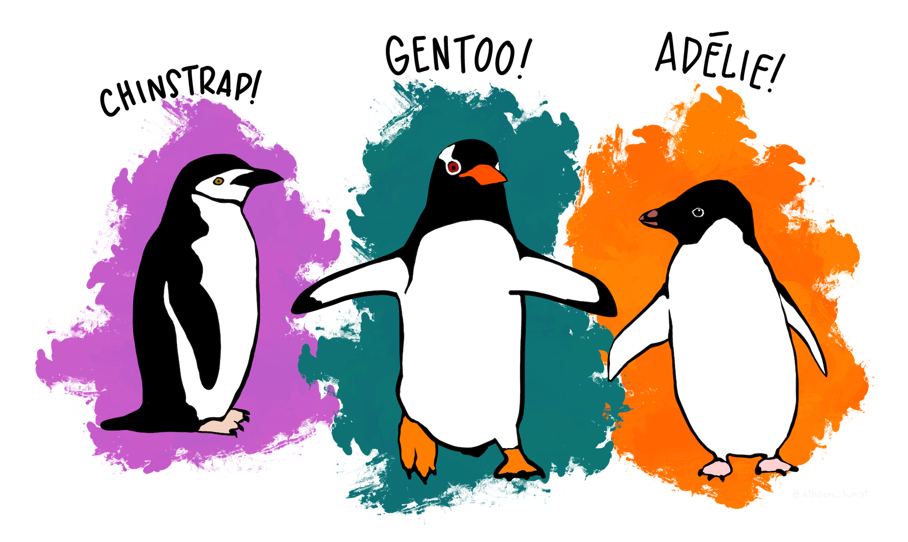
The Palmer Penguins dataset is a widely used open dataset in data science and machine learning education. These data were collected from 2007 - 2009 by Dr. Kristen Gorman with the Palmer Station Long Term Ecological Research Program, part of the US Long Term Ecological Research Network. It contains measurements for 344 penguins from three species – Adelie, Chinstrap, and Gentoo – collected from three islands (Biscoe, Dream, and Torgersen) in the Palmer Archipelago, Antarctica.
The data were imported directly from the Environmental Data Initiative (EDI) Data Portal, and are available for use by CC0 license (“No Rights Reserved”) in accordance with the Palmer Station Data Policy.
from IPython.display import Image, display
display(Image("../images/numerical-data/penguins.png", width=1240))
1.1 Loading dataset
Seaborn provides the Penguins dataset through its built-in data-loading functions. We can access it using sns.load_dataset('penguin') and then have a quick look at the data.
Note
If you have your own dataset stored in a CSV file, you can easily load it into Python using Pandas with the read_csv() function. This is one of the most common ways to bring tabular data into a DataFrame for further analysis and processing.
Beyond CSV files, Pandas also supports a wide variety of other file formats, making it a powerful and flexible tool for data handling. For example, you can use read_excel() to import data from Microsoft Excel spreadsheets, read_hdf() to work with HDF5 binary stores, and read_json() to load data from JSON files. Each of these formats also has a corresponding method for saving data back to disk, such as to_csv(), to_excel(), to_hdf(), and to_json().
import numpy as np
import pandas as pd
import matplotlib.pyplot as plt
import seaborn as sns
# penguins = pd.read_csv("./penguins_dataset.csv")

# URL of Penguins dataset (CSV file)
# url = "https://raw.githubusercontent.com/mwaskom/seaborn-data/master/penguins.csv"
# penguins = pd.read_csv(url)

penguins = sns.load_dataset('penguins')
penguins
| species | island | bill_length_mm | bill_depth_mm | flipper_length_mm | body_mass_g | sex | |
|---|---|---|---|---|---|---|---|
| 0 | Adelie | Torgersen | 39.1 | 18.7 | 181.0 | 3750.0 | Male |
| 1 | Adelie | Torgersen | 39.5 | 17.4 | 186.0 | 3800.0 | Female |
| 2 | Adelie | Torgersen | 40.3 | 18.0 | 195.0 | 3250.0 | Female |
| 3 | Adelie | Torgersen | NaN | NaN | NaN | NaN | NaN |
| 4 | Adelie | Torgersen | 36.7 | 19.3 | 193.0 | 3450.0 | Female |
| ... | ... | ... | ... | ... | ... | ... | ... |
| 339 | Gentoo | Biscoe | NaN | NaN | NaN | NaN | NaN |
| 340 | Gentoo | Biscoe | 46.8 | 14.3 | 215.0 | 4850.0 | Female |
| 341 | Gentoo | Biscoe | 50.4 | 15.7 | 222.0 | 5750.0 | Male |
| 342 | Gentoo | Biscoe | 45.2 | 14.8 | 212.0 | 5200.0 | Female |
| 343 | Gentoo | Biscoe | 49.9 | 16.1 | 213.0 | 5400.0 | Male |
344 rows × 7 columns
1.2 Getting statistics
Once we have imported the Penguins dataset, our first step is to understand which columns contain numerical data. In this dataset, there are seven columns. Variables such as bill_length_mm, bill_depth_mm, flipper_length_mm, and body_mass_g are numerical, while columns such as species, island, and sex are categorical.
penguins.info()
<class 'pandas.DataFrame'>
RangeIndex: 344 entries, 0 to 343
Data columns (total 7 columns):
 #   Column             Non-Null Count  Dtype
---  ------             --------------  -----
 0   species            344 non-null    str
 1   island             344 non-null    str
 2   bill_length_mm     342 non-null    float64
 3   bill_depth_mm      342 non-null    float64
 4   flipper_length_mm  342 non-null    float64
 5   body_mass_g        342 non-null    float64
 6   sex                333 non-null    str
dtypes: float64(4), str(3)
memory usage: 18.9 KB
For columns with numverical variables, we can summarize using statistics such as the mean, median, minimum, maximum, and standard deviation via .describe().
penguins.describe()
| bill_length_mm | bill_depth_mm | flipper_length_mm | body_mass_g | |
|---|---|---|---|---|
| count | 342.000000 | 342.000000 | 342.000000 | 342.000000 |
| mean | 43.921930 | 17.151170 | 200.915205 | 4201.754386 |
| std | 5.459584 | 1.974793 | 14.061714 | 801.954536 |
| min | 32.100000 | 13.100000 | 172.000000 | 2700.000000 |
| 25% | 39.225000 | 15.600000 | 190.000000 | 3550.000000 |
| 50% | 44.450000 | 17.300000 | 197.000000 | 4050.000000 |
| 75% | 48.500000 | 18.700000 | 213.000000 | 4750.000000 |
| max | 59.600000 | 21.500000 | 231.000000 | 6300.000000 |
For example, if we look at body_mass_g, we might see that the mean is somewhere around 4,200 grams. This tells us the average body mass of the penguins in the available observations. The minimum and maximum tell us the range of observed body masses, while the quartiles tell us how the observations are distributed within that range.
Quartiles divide the ordered data into sections. The 25th percentile, or Q1, tells us the value below which approximately 25% of observations fall. The median divides the data in half, and Q3 marks approximately the 75th percentile. The distance between Q1 and Q3 is called the interquartile range (IQR). The IQR is useful because it describes the spread of the middle 50% of our observations and is less influenced by extreme values.
If the mean and median (50%) are relatively close, that can suggest that the distribution is reasonably balanced. If they are noticeably different, it may indicate that the data is skewed or that some unusually large or small observations are affecting the mean.
1.3 Data visualization
Looking only at the raw numbers in the penguins DataFrame, or even examining the statistical summaries provided by penguins.info() and penguins.describe(), often does not give us a clear intuition about the patterns and relationships in the data. To truly understand the dataset, we generally prefer to visualize the data, since graphical representations can reveal trends, groupings, and anomalies that may remain hidden in numerical summaries alone.
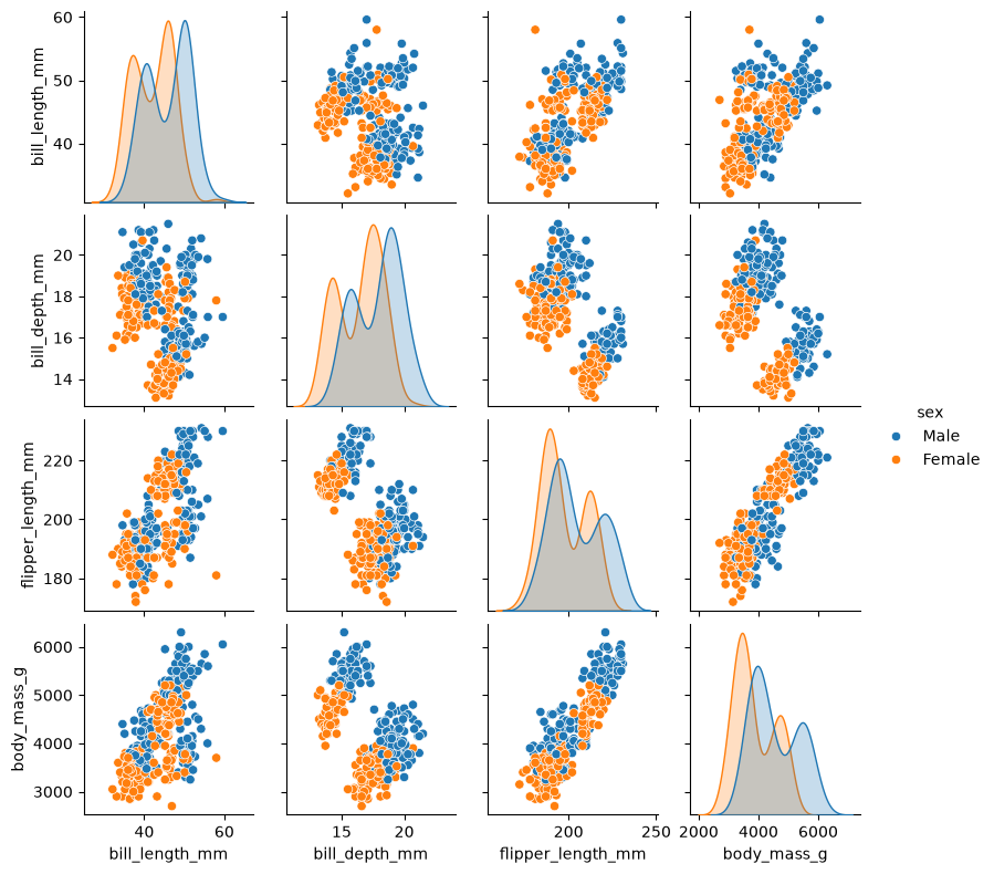
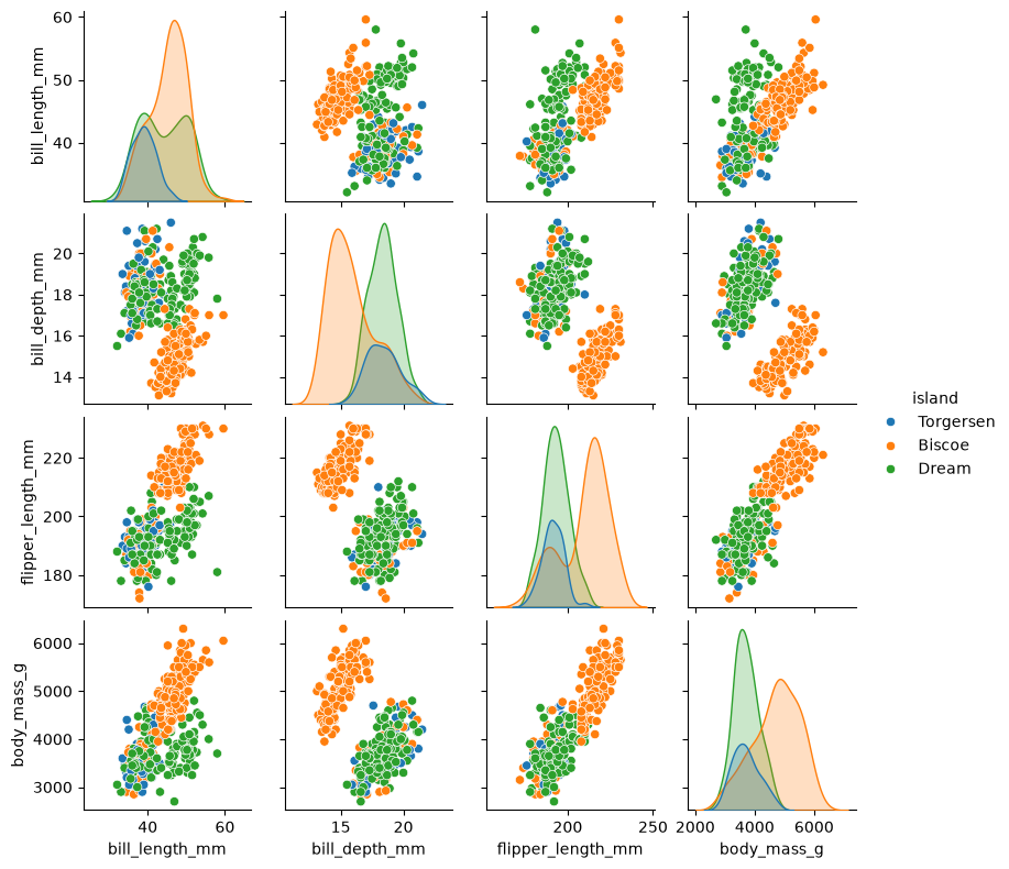
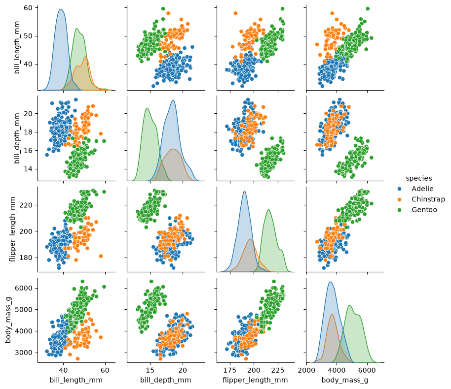
One nice visualization for datasets with relatively few attributes is Pair Plot, which can be created using sns.pairplot(...). It shows a scatterplot of each attribute plotted against each of the other attributes. By using the hue='species' setting for the pairplot the graphs on the diagonal are layered kernel density estimate plots for the different values of the species column.
sns.pairplot(penguins, hue="sex", height=2.0)
<seaborn.axisgrid.PairGrid at 0x16ddbe690>
sns.pairplot(penguins, hue="island", height=2.0)
<seaborn.axisgrid.PairGrid at 0x148507690>
sns.pairplot(penguins, hue="species", height=2.0)
<seaborn.axisgrid.PairGrid at 0x1480a6690>
Discussion
Take a look at the pairplot we created. Consider the following questions:
Is there any class that is easily distinguishable from the others?
Which combination of attributes shows the best separation for all 3 class labels at once?
For pairplot with
hue="sex", which combination of features distinguishes the two sexes best?What about the one with
hue="island"?
2. Imputating Missing Values
After getting a statistical overview of our numerical variables, the next issue we need to investigate is missing data. In a real-world dataset, it is common for some measurements to be unavailable. In the Penguins dataset, for example, some penguins may have a missing body_mass_g, flipper_length_mm, or another measurement.
Missing values matter because many calculations and machine-learning algorithms cannot work directly with incomplete data. Before deciding what to do with missing values, however, we first need to find them and understand how much data is actually missing. The important point is that we should inspect the missing data before automatically deleting or replacing anything.
# check whether each column contains missing values
penguins.isna().sum()
species               0
island                0
bill_length_mm        2
bill_depth_mm         2
flipper_length_mm     2
body_mass_g           2
sex                  11
dtype: int64
To focus specifically on numerical columns:
numericals = ["body_mass_g", "bill_length_mm", "bill_depth_mm", "flipper_length_mm"]
penguins_numericals = penguins[numericals].copy()
penguins_numericals
| body_mass_g | bill_length_mm | bill_depth_mm | flipper_length_mm | |
|---|---|---|---|---|
| 0 | 3750.0 | 39.1 | 18.7 | 181.0 |
| 1 | 3800.0 | 39.5 | 17.4 | 186.0 |
| 2 | 3250.0 | 40.3 | 18.0 | 195.0 |
| 3 | NaN | NaN | NaN | NaN |
| 4 | 3450.0 | 36.7 | 19.3 | 193.0 |
| ... | ... | ... | ... | ... |
| 339 | NaN | NaN | NaN | NaN |
| 340 | 4850.0 | 46.8 | 14.3 | 215.0 |
| 341 | 5750.0 | 50.4 | 15.7 | 222.0 |
| 342 | 5200.0 | 45.2 | 14.8 | 212.0 |
| 343 | 5400.0 | 49.9 | 16.1 | 213.0 |
344 rows × 4 columns
2.1 Dropping missing observations
Sometimes we only care about missing values in a particular numerical variable. For example, suppose we want to find the observations where the body mass value is missing. We can filter the dataset based on the missing values in the other columns. This is useful because it allows us to inspect the actual observations rather than treating missing values as abstract numbers.
At this point, we should ask an important question: Should we delete these rows, or should we fill in the missing values? One straightforward approach is to remove rows containing missing values. Pandas provides .dropna() for this.
print("Original shape:", penguins_numericals.shape)
penguins_numericals_dropna = penguins_numericals.dropna()
print("New shape:", penguins_numericals_dropna.shape)
Original shape: (344, 4)
New shape: (342, 4)
Warning
The dropna() is easy to use, but “easy” does not necessarily mean “appropriate”.
The decision to drop rows should therefore depend on the situation. If only a small number of observations are missing and those observations are not critical, dropping them may be perfectly reasonable. But if many observations are missing, deleting them could significantly reduce our dataset and potentially introduce bias.
2.2 Imputation of missing values
Another option is to impute the missing values with a suitable estimate. Common choices include the mean or median of that column, depending on the distribution.
Here we calculate mean and median values for numerical features. To illustrate this process, we take body_mass_g feature as an example.
body_mass_g_mean = penguins_numericals.body_mass_g.mean()
body_mass_g_median = penguins_numericals.body_mass_g.median()
print(f"  mean value of body_mass_g is {body_mass_g_mean}")
print(f"median value of body_mass_g is {body_mass_g_median}")
  mean value of body_mass_g is 4201.754385964912
median value of body_mass_g is 4050.0
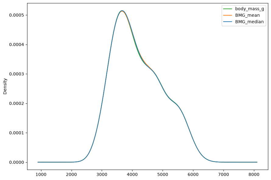
Rather than directly replacing missing values, we concatenate new columns containing mean and median values for the body_mass_g feature to end of Penguins dataset, and than visualize distribution of this feature.
penguins_numericals['BMG_mean'] = penguins_numericals.body_mass_g.fillna(body_mass_g_mean)
penguins_numericals['BMG_median'] = penguins_numericals.body_mass_g.fillna(body_mass_g_median)
penguins_numericals.head().style.highlight_null(color = 'green')
| body_mass_g | bill_length_mm | bill_depth_mm | flipper_length_mm | BMG_mean | BMG_median | |
|---|---|---|---|---|---|---|
| 0 | 3750.000000 | 39.100000 | 18.700000 | 181.000000 | 3750.000000 | 3750.000000 |
| 1 | 3800.000000 | 39.500000 | 17.400000 | 186.000000 | 3800.000000 | 3800.000000 |
| 2 | 3250.000000 | 40.300000 | 18.000000 | 195.000000 | 3250.000000 | 3250.000000 |
| 3 | nan | nan | nan | nan | 4201.754386 | 4050.000000 |
| 4 | 3450.000000 | 36.700000 | 19.300000 | 193.000000 | 3450.000000 | 3450.000000 |
plt.figure(figsize=(9, 6))

penguins_numericals['body_mass_g'].plot(kind='kde', color='tab:green', label="body_mass_g")
penguins_numericals['BMG_mean'].plot(kind='kde', color='tab:orange', label="BMG_mean")
penguins_numericals['BMG_median'].plot(kind='kde', color='tab:blue', label="BMG_median")

plt.legend(loc='best')
plt.tight_layout()
Mean or median imputation
Mean imputation is simple and can work well when the data is reasonably balanced and the missing values are not strongly associated with unusual observations.
But there is an important limitation: the mean can be affected by extreme values. If a numerical variable is strongly skewed or contains outliers, the mean may not represent a typical observation very well.
In such situation, the median becomes particularly useful. The median is less sensitive to extreme values than the mean, so it can often be a better choice when numerical data is skewed or contains outliers.
The key lesson is that missing-value handling is not simply a technical step. We need to make a decision based on how much data is missing, where it is missing, and what effect removing or replacing it might have on our analysis.
3. Handling Outliers
After getting statistical information from the Penguins dataset, the next step is to look more carefully at the unusual observations.
An outlier is a value that is unusually far from the other observations. For instance, if body mass of most of penguins in dataset varies between 3000-6000 g, an observation of 7500 g will be considered as an outlier since such an observation occurs rarely.
Outliers can occur because of measurement errors, data-entry mistakes, unusual but genuine cases, or because the population itself naturally contains extreme observations. Therefore, we should not automatically delete an outlier just because it looks unusual. Instead, we first identify it, investigate it, understand its impact, and then decide whether to retain, remove, or transform it.
penguins_numericals
| body_mass_g | bill_length_mm | bill_depth_mm | flipper_length_mm | BMG_mean | BMG_median | |
|---|---|---|---|---|---|---|
| 0 | 3750.0 | 39.1 | 18.7 | 181.0 | 3750.000000 | 3750.0 |
| 1 | 3800.0 | 39.5 | 17.4 | 186.0 | 3800.000000 | 3800.0 |
| 2 | 3250.0 | 40.3 | 18.0 | 195.0 | 3250.000000 | 3250.0 |
| 3 | NaN | NaN | NaN | NaN | 4201.754386 | 4050.0 |
| 4 | 3450.0 | 36.7 | 19.3 | 193.0 | 3450.000000 | 3450.0 |
| ... | ... | ... | ... | ... | ... | ... |
| 339 | NaN | NaN | NaN | NaN | 4201.754386 | 4050.0 |
| 340 | 4850.0 | 46.8 | 14.3 | 215.0 | 4850.000000 | 4850.0 |
| 341 | 5750.0 | 50.4 | 15.7 | 222.0 | 5750.000000 | 5750.0 |
| 342 | 5200.0 | 45.2 | 14.8 | 212.0 | 5200.000000 | 5200.0 |
| 343 | 5400.0 | 49.9 | 16.1 | 213.0 | 5400.000000 | 5400.0 |
344 rows × 6 columns
3.1 Imputating missing values with extreme data
In the code snippet below, we create a new column for body_mass_g and impute its missing values using the extreme end of the distribution (EoD). Here, the EoD is defined as the mean plus three standard deviations, calculated as mean + (3 * std).
eod_value = penguins['body_mass_g'].mean() + 3 * penguins['body_mass_g'].std() + 200
print(eod_value)

penguins_numericals['species'] = penguins['species']
penguins_numericals['BMG_EoD'] = penguins_numericals['body_mass_g'].fillna(eod_value)
penguins_numericals.head(5).style.highlight_null(color = 'green')
6807.617993059199
| body_mass_g | bill_length_mm | bill_depth_mm | flipper_length_mm | BMG_mean | BMG_median | species | BMG_EoD | |
|---|---|---|---|---|---|---|---|---|
| 0 | 3750.000000 | 39.100000 | 18.700000 | 181.000000 | 3750.000000 | 3750.000000 | Adelie | 3750.000000 |
| 1 | 3800.000000 | 39.500000 | 17.400000 | 186.000000 | 3800.000000 | 3800.000000 | Adelie | 3800.000000 |
| 2 | 3250.000000 | 40.300000 | 18.000000 | 195.000000 | 3250.000000 | 3250.000000 | Adelie | 3250.000000 |
| 3 | nan | nan | nan | nan | 4201.754386 | 4050.000000 | Adelie | 6807.617993 |
| 4 | 3450.000000 | 36.700000 | 19.300000 | 193.000000 | 3450.000000 | 3450.000000 | Adelie | 3450.000000 |
plt.figure(figsize=(8, 5))

sns.swarmplot(y=penguins_numericals["species"], x=penguins_numericals["BMG_EoD"],
              color="lightgreen", marker="o", size=4)

sns.boxplot(y=penguins_numericals["species"], x=penguins_numericals["BMG_EoD"],
            palette="coolwarm", notch=True, linewidth=2, width=0.5,
            hue=penguins_numericals.species, legend=False)

plt.xlabel("Body mass (g)", fontsize=14)
plt.ylabel("Species", fontsize=14)
plt.tick_params(axis='x', labelsize=12)
plt.tick_params(axis='y', labelsize=12)

plt.tight_layout()
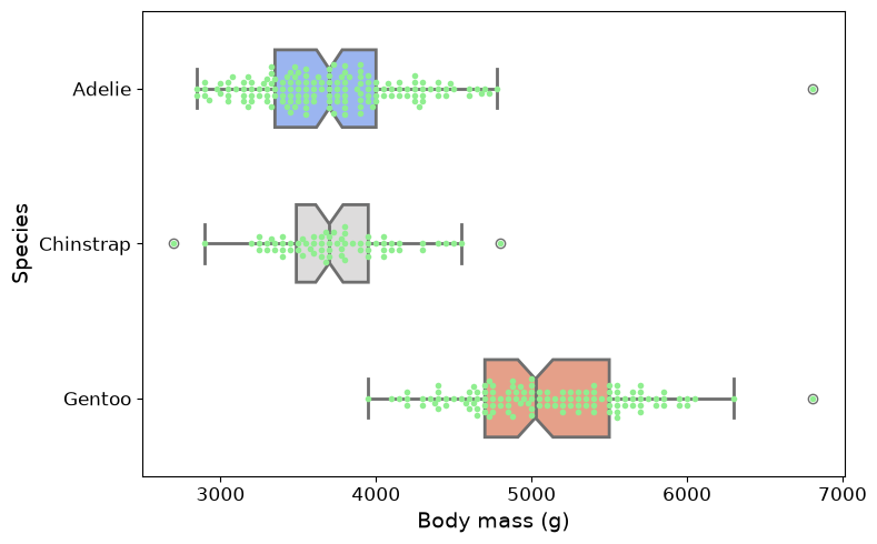
There are several approaches to identify outliers, and two of most commonly used methods are Interquartile Range (IQR) method and Mean-Standard Deviation method.
3.2 The Inter quartile range (IQR) method
penguins_numericals.body_mass_g.describe()
count     342.000000
mean     4201.754386
std       801.954536
min      2700.000000
25%      3550.000000
50%      4050.000000
75%      4750.000000
max      6300.000000
Name: body_mass_g, dtype: float64
IQR measures spread of middle 50% of data and is calculated by subtracting 1st quartile (25th percentile, Q1) from 3rd quartile (75th percentile, Q3).
Once IQR is obtained, we can determine boundaries for detecting outliers.
Lower limit is defined as Q1 minus 1.5 times IQR.
Upper limit is defined as Q3 plus 1.5 times IQR.
print(f"25% quantile = {penguins_numericals['body_mass_g'].quantile(0.25)}")
print(f"75% quantile = {penguins_numericals['body_mass_g'].quantile(0.75)}\n")

IQR = penguins_numericals["body_mass_g"].quantile(0.75) - penguins_numericals["body_mass_g"].quantile(0.25)
lower_bmg_limit = penguins_numericals["body_mass_g"].quantile(0.25) - (1.5 * IQR)
upper_bmg_limit = penguins_numericals["body_mass_g"].quantile(0.75) + (1.5 * IQR)

print(f"lower limt of IQR = {lower_bmg_limit} and upper limit of IQR = {upper_bmg_limit}")
25% quantile = 3550.0
75% quantile = 4750.0

lower limt of IQR = 1750.0 and upper limit of IQR = 6550.0
Any data points that fall below lower limit or above upper limit are considered outliers, and these points are subsequently removed from dataset.
# check data points larger than upper limit of IQR range
penguins_numericals[penguins_numericals["BMG_EoD"] > upper_bmg_limit]
| body_mass_g | bill_length_mm | bill_depth_mm | flipper_length_mm | BMG_mean | BMG_median | species | BMG_EoD | |
|---|---|---|---|---|---|---|---|---|
| 3 | NaN | NaN | NaN | NaN | 4201.754386 | 4050.0 | Adelie | 6807.617993 |
| 339 | NaN | NaN | NaN | NaN | 4201.754386 | 4050.0 | Gentoo | 6807.617993 |
# check data points smaller than lower limit of IQR range
penguins_numericals[penguins_numericals["body_mass_g"] < lower_bmg_limit]
| body_mass_g | bill_length_mm | bill_depth_mm | flipper_length_mm | BMG_mean | BMG_median | species | BMG_EoD |
|---|
What should we actually do with the outliers?
It is tempting to say, “We found outliers, so let’s delete them.” But that isn’t necessarily the right decision.
Imagine that an unusually heavy penguin is a genuine measurement.
Removing it would mean throwing away valid information.
On the other hand, if we discover that a measurement was entered incorrectly. For example, 35,000 grams instead of 3,500 grams, then removing or correcting that observation may be appropriate.
The decision can be thought of as three possibilities:
Retain: The value is unusual but valid.
Remove: The value is incorrect, impossible, or inappropriate for the analysis.
Transform or cap: The value is valid, but its extreme magnitude has too much influence on the analysis.
Capping or winsorizing
Instead of deleting extreme observations, another option is to cap them. This means we keep the observation but limit its value to a predefined boundary.
For the two abnormal values in
BMG_EoDcolumn, values below the lower boundary are replaced by the lower boundary, and values above the upper boundary are replaced by the upper boundary.This approach is sometimes called winsorizing when extreme values are replaced with specified percentile-based limits.
The advantage is that we don’t lose entire observations.
The disadvantage is that we are changing the numerical values, so we need to make sure that this transformation makes sense for our particular analysis.
4. Scaling & Normalizing Numerical Data
In many datasets, numerical features can be measured in very different units and ranges. For example, in the Penguins dataset, body mass is measured in grams and can range in the thousands, while flipper length is measured in millimeters and typically ranges in the hundreds. Both are numerical variables, but their numerical scales are very different. This difference can matter when we use the data for certain types of analysis and machine learning, making features with larger values dominate the learning process, leading to biased and inaccurate models.
Scaling transforms these features to a common, limited range, such as [0, 1] or a distribution with a mean of 0 and a standard deviation of 1, without distorting the differences in the ranges of values or losing information.
In this section, we will apply two common methods, standardization (Z-score normalization) and normalization (min-max scaling), to tranform the data.
4.1 Standardization (Z-score Normalization)
One of the most common approaches is standardization. Standardization transforms a variable so that it has a mean close to 0 and a standard deviation close to 1. It is calculated by subtracting the mean value ($\mu$) of the feature and then dividing by the standard deviation ($\sigma$), and its formula is $X_scaled = \frac{X - \mu}{\sigma}$.
penguins_BMG = penguins[["body_mass_g"]].copy()
penguins_BMG.dropna(inplace=True)
print(penguins_BMG)
     body_mass_g
0         3750.0
1         3800.0
2         3250.0
4         3450.0
5         3650.0
..           ...
338       4925.0
340       4850.0
341       5750.0
342       5200.0
343       5400.0

[342 rows x 1 columns]
We use the StandardScaler from scikit-learn to standardize the body_mass_g variable. It transforms the data by subtracting the mean and dividing by the standard deviation, resulting in a mean of approximately 0 and a standard deviation of 1. This ensures that the variable is on a consistent scale for machine learning algorithms.
from sklearn.preprocessing import StandardScaler
scaler = StandardScaler()
penguins_BMG["BMG_Std"] = scaler.fit_transform(penguins_BMG[["body_mass_g"]])
penguins_BMG
| body_mass_g | BMG_Std | |
|---|---|---|
| 0 | 3750.0 | -0.564142 |
| 1 | 3800.0 | -0.501703 |
| 2 | 3250.0 | -1.188532 |
| 4 | 3450.0 | -0.938776 |
| 5 | 3650.0 | -0.689020 |
| ... | ... | ... |
| 338 | 4925.0 | 0.903175 |
| 340 | 4850.0 | 0.809516 |
| 341 | 5750.0 | 1.933419 |
| 342 | 5200.0 | 1.246590 |
| 343 | 5400.0 | 1.496346 |
342 rows × 2 columns
# verify mean and standard deviation of standardized BMG data
print("mean value:", penguins_BMG["BMG_Std"].mean())
print("standard deviation:", penguins_BMG["BMG_Std"].std())
mean value: 4.15522067695965e-17
standard deviation: 1.0014652022510058
4.2 Normalization (Min-Max Scaling)
Standardization is not the only option. Another common approach is min-max normalization, which transforms values into a specified range, typically [0, 1]. It is calculated by subtracting the minimum value of the feature and then dividing by the range (max - min), and its formula is $X_scaled = \frac{(X - X_min)}{(X_max - X_min)}$.
This method is useful when the distribution is not Gaussian or when the algorithm requires input values bounded within a specific range (e.g., neural networks often use activation functions that expect inputs in the [0,1] range).
from sklearn.preprocessing import MinMaxScaler
minmax_scaler = MinMaxScaler()
penguins_BMG["BMG_MinMax"] = minmax_scaler.fit_transform(penguins_BMG[["body_mass_g"]])
penguins_BMG
| body_mass_g | BMG_Std | BMG_MinMax | |
|---|---|---|---|
| 0 | 3750.0 | -0.564142 | 0.291667 |
| 1 | 3800.0 | -0.501703 | 0.305556 |
| 2 | 3250.0 | -1.188532 | 0.152778 |
| 4 | 3450.0 | -0.938776 | 0.208333 |
| 5 | 3650.0 | -0.689020 | 0.263889 |
| ... | ... | ... | ... |
| 338 | 4925.0 | 0.903175 | 0.618056 |
| 340 | 4850.0 | 0.809516 | 0.597222 |
| 341 | 5750.0 | 1.933419 | 0.847222 |
| 342 | 5200.0 | 1.246590 | 0.694444 |
| 343 | 5400.0 | 1.496346 | 0.750000 |
342 rows × 3 columns
# verify min and max values of normalized BMG data
print("min value:", penguins_BMG["BMG_MinMax"].min())
print("max value:", penguins_BMG["BMG_MinMax"].max())
min value: 0.0
max value: 1.0
Normalization vs. Standardization
Normalization, such as Min-Max scaling, is useful when features need to be mapped to a specific range, typically between 0 and 1, but it can be sensitive to outliers because extreme values affect the minimum and maximum.
Standardization transforms data to have a mean of 0 and a standard deviation of 1, making it generally more robust to differences in feature scales, and is less affected by outliers, although it does not restrict values to a fixed range.
Both methods can improve model performance and convergence, but the appropriate choice depends on the data distribution and the requirements of the machine learning algorithm.
Exercise
After completing the individual tasks for handling numerical data, it is now time to bring everything together in a hands-on exercise. In this activity, we will work with representative datasets from scikit-learn and apply the data-handling techniques we have learned throughout the episode.
Select a dataset: Choose one dataset from scikit-learn: Iris, Diabetes, Wine, Breast Cancer, or California Housing.
from sklearn import datasets

iris = datasets.load_iris(as_frame=True)
iris_df = iris.frame
iris_df.head()

diabetes = datasets.load_diabetes(as_frame=True)
diabetes_df = diabetes.frame
diabetes_df.head()

wine = datasets.load_wine(as_frame=True)
wine_df = wine.frame
wine_df.head()

cancer = datasets.load_breast_cancer(as_frame=True)
cancer_df = cancer.frame
cancer_df.head()

housing = datasets.fetch_california_housing(as_frame=True)
housing_df = housing.frame
housing_df.head()
Inspect the dataset: Examine the shape, columns, data types, and first few observations.
Remove unnecessary rows and columns: Identify irrelevant or redundant data and remove it where appropriate.
Get statistical information: Calculate and interpret count, mean, median, minimum, maximum, quartiles, and standard deviation.
Check for missing values: Identify missing values and calculate their counts and percentages.
Decide how to handle missing values: Determine whether to remove observations or impute missing numerical values using an appropriate method.
Identify and handle outliers: Use summary statistics, the IQR method, and visualizations to identify potential outliers, then decide whether to retain, remove, or cap them.
Scale or normalize numerical features: Apply standardization or min-max normalization to selected features and compare the values before and after transformation.
Verify the cleaned dataset: Check the final shape, columns, data types, missing values, ranges, and other relevant properties to confirm that the dataset is ready for further analysis or machine learning.
Keypoints
Get familiar with the Palmer Penguins dataset.
Perform statistical analysis and data visualization using Pandas and Seaborn.
Identify and handle missing values in numerical features.
Identify and handle outliers in the dataset.
Apply standardization and normalization techniques to numerical features.