Heat diffusion mini-app

Questions

• How can I learn about OpenMP on GPUs with a practical example?

• What should I think about when porting code to use GPUs?

Objectives

• Understand the structure of a mini-app that models heat diffusion

• Understand how the 5-point stencil operates

• Understand that the loops influence the duration of the mini-app

• Understand the expected output of the mini-app

Prerequisites

1. Understanding of how to read either C++ or Fortran code

2. Running programs from a terminal command line

Heat diffusion

Heat flows in objects according to local temperature differences, as if seeking local equilibrium. Such processes can be modelled with partial differential equations via discretization to a regular grid. Solving for the flow over time can involve a lot of computational effort. Fortunately that effort is quite regular and so can suit parallelization with a variety of techniques. That includes OpenMP offload to GPUs, so first we will introduce this mini-app and then use it to explore OpenMP offload The mini-app is based on one developed by CSC in Finland, and is used here with permission granted by their license.

The partial differential equation

The rate of change of the temperature field \(u(x, y, t)\) over two spatial dimensions \(x\) and \(y\) and time \(t\) with diffusivity \(\alpha\) can be modelled via the equation

\[\frac{\partial u}{\partial t} = \alpha \nabla^2 u\]

where \(\nabla\) is the Laplacian operator, which describes how the temperature field varies with the spatial dimensions \(x\) and \(y\). When those are continuous variables, that looks like

\[\frac{\partial u}{\partial t} = \alpha \left( \frac{\partial^2 u}{\partial x^2} + \frac{\partial^2 u}{\partial x^2}\right)\]

Because computers are finite devices, we often need to solve such equations numerically, rather than analytically. This often involves discretization, where spatial and temporal variables only take on specific values from a set. In this mini-app we will discretize all three dimensions \(x\), \(y\), and \(t\), such that

\[\begin{split}\nabla^2 u &= \frac{u(i-1,j)-2u(i,j)+u(i+1,j)}{(\Delta x)^2} \\ &+ \frac{u(i,j-1)-2u(i,j)+u(i,j+1)}{(\Delta y)^2}\end{split}\]

where \(u(i,j)\) refers to the temperature at location with integer index \(i\) within the domain of \(x\) spaced by \(\Delta x\) and location with integer index \(j\) within the domain of \(y\) spaced by \(\Delta y\).

Given an initial condition \((u^{t=0})\), one can follow the time dependence of the temperature field from state \(m\) to \(m+1\) over regular time steps \(\Delta t\) with explicit time evolution method:

\[u^{m+1}(i,j) = u^m(i,j) + \Delta t \alpha \nabla^2 u^m(i,j)\]

This equation expresses that the time evolution of the temperature field at a particular location depends on the value of the field at the previous step at the same location and four adjacent locations:

This example model uses an 8x8 grid of data in light blue in state \(m\), each location of which has to be updated based on the indicated 5-point stencil in yellow to move to the next time point \(m+1\).

Exercise

How much arithmetic must be done to evolve each location at each time step?

Solution

10 arithmetic operations per location per time step. 3 in each of 2 numerators, 1 to divide by each pre-computed denominator, and two additions to update \(u\).

Exercise

How much arithmetic must be done to evolve all locations in the grid for 20 steps?

Solution

There’s 64 locations and 20 steps and each does the same 10 operations, so \(10*8*8*20 = 12800\) arithmetic operations total. However, that assumes that there are no boundaries to the field, which is unrealistic!

Spatial boundary conditions

Something must happen at the edges of the grid so that the stencil does a valid operation. One alternative is to ignore the contribution of points that are outside the grid. However, this tends to complicate the implementation of the stencil and is also often non-physical. In a real problem, there is always something outside the grid! Sometimes it makes sense to have periodic boundaries to the grid, but that is complex to implement. In this mini-app, we will have a ring of data points around the grid. Those will have a fixed value that is not updated by the stencil, although they do contribute to the stencil operation for their neighbors.

This example model uses an 8x8 grid of data in light blue with an outer ring in red of boundary grid sites whose temperature values are fixed. This lets the stencil operate on the blue region in a straightforward way.

The source code

Now we’ll take a look at the source code that will do this for us! Let’s look at the data structure describing the field:

The field data structure

C++Fortran

struct field {
    // nx and ny are the dimensions of the field. The array data
    // contains also ghost layers, so it will have dimensions nx+2 x ny+2
    int nx;
    int ny;
    // Size of the grid cells
    double dx;
    double dy;
    // The temperature values in the 2D grid
    std::vector<double> data;
};

Next, the routine that applies the stencil to the previous field to compute the current one:

The core evolution operation

C++Fortran

// Update the temperature values using five-point stencil
// Arguments:
//   curr: current temperature values
//   prev: temperature values from previous time step
//   a: diffusivity
//   dt: time step
void evolve(field *curr, field *prev, double a, double dt)
{
  // Help the compiler avoid being confused by the structs
  double *currdata = curr->data.data();
  double *prevdata = prev->data.data();
  int nx = curr->nx;
  int ny = curr->ny;

  // Determine the temperature field at next time step
  // As we have fixed boundary conditions, the outermost gridpoints
  // are not updated.
  double dx2 = prev->dx * prev->dx;
  double dy2 = prev->dy * prev->dy;
  for (int i = 1; i < nx + 1; i++) {
    for (int j = 1; j < ny + 1; j++) {
      int ind = i * (ny + 2) + j;
      int ip = (i + 1) * (ny + 2) + j;
      int im = (i - 1) * (ny + 2) + j;
      int jp = i * (ny + 2) + j + 1;
      int jm = i * (ny + 2) + j - 1;
      currdata[ind] = prevdata[ind] + a*dt*
	    ((prevdata[ip] - 2.0*prevdata[ind] + prevdata[im]) / dx2 +
	     (prevdata[jp] - 2.0*prevdata[ind] + prevdata[jm]) / dy2);
    }
  }
}

Then the routine that handles the main loop over time steps:

The main driver function

C++Fortran

int main(int argc, char **argv)
{
    // Number of time steps
    int nsteps;
    // Current and previous temperature fields
    field current, previous;
    initialize(argc, argv, &current, &previous, &nsteps);

    // Diffusion constant
    double a = 0.5;

    // Compute the largest stable time step
    double dx2 = current.dx * current.dx;
    double dy2 = current.dy * current.dy;
    // Time step
    double dt = dx2 * dy2 / (2.0 * a * (dx2 + dy2));

    // Time evolution
    for (int iter = 1; iter <= nsteps; iter++) {
        evolve(&current, &previous, a, dt);
        // Swap current field so that it will be used
        // as previous for next iteration step
        swap_fields(&current, &previous);
    }

}

There’s other supporting code to handle user input and produce nice images of the current field, but we won’t need to touch those, so we won’t spend time looking at them now. In the real version of the code we have seen, there’s also calls to libraries to record the time taken. We’ll need that later so we understand how fast our code is.

We should look at the routines that initialize the field data structures:

The setup routines

C++Fortran

// Allocate memory for a temperature field and initialise it to zero
void allocate_field(field *temperature)
{
    // Include also boundary layers
    int newSize = (temperature->nx + 2) * (temperature->ny + 2);
    temperature->data.resize(newSize, 0.0);
}

Building the code

The code is set up so that you can change to its directory, type make and it will build and run for you.

Building the code

C++Fortran

cd content/exercise/serial
make

You will see output something like:

nvc++ -g -O3 -fopenmp -Wall -I../common -c main.cpp -o main.o
nvc++ -g -O3 -fopenmp -Wall -I../common -c core.cpp -o core.o
nvc++ -g -O3 -fopenmp -Wall -I../common -c setup.cpp -o setup.o
nvc++ -g -O3 -fopenmp -Wall -I../common -c utilities.cpp -o utilities.o
nvc++ -g -O3 -fopenmp -Wall -I../common -c io.cpp -o io.o
nvc++ -g -O3 -fopenmp -Wall -I../common main.o core.o setup.o utilities.o io.o ../common/pngwriter.o -o heat_serial  -lpng

which produces an executable program called heat_serial.

Running the code

The code lets you choose the spatial dimensions and the number of time steps on the command line. For example, to run an 800 by 800 grid for 1000 steps, run

./heat_serial 800 800 1000

Try it now!

Exercise

How long does the iteration take if you double the number of steps? How long does the iteration take if you double the number of grid points in each direction?

Solution

Doubling the number of steps doubles the total amount of work, so should take around twice as long. Doubling both numbers of grid points is four times as much work, so should take around four times as long.

You can see the output on the terminal, like:

Average temperature at start: 59.762281
Iterations took 0.426 seconds.
Average temperature: 58.065097

This report will help us check whether our attempts to optimize made the code faster while keeping it correct.

Initial and boundary conditions

When solving PDEs, the initial conditions determine the possible solutions. The mini-app automatically sets up a disk of cold grid points in the center at temperature 5, with warm grid points around it at temperature 65.

Initial conditions of the grid. The boundary layers are not shown.

There is a fixed boundary layer of one grid point on all sides, two of which are warm (temperature 70 and 85) and two cold (temperature 20 and 5). Early on, the disk and its surroundings dominate the contents of the grid, but over time, the boundary layers have greater and greater influence.

Exercise

To which average temperature will the grid converge?

Solution

Eventually, the boundary conditions will dominate. Each contributes equally if the sides are of equal length. The average of the grid will be the average of the boundaries, ie. \((70+20+85+5)/4\) which is \(45\).

Visualizing the output

The mini-app has support for writing an image file that shows the state of the grid every 1500 steps. Below we can see the progression over larger numbers of steps:

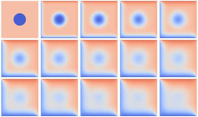
Over time, the grid progresses from the initial state toward an end state where one triangle is cold and one is warm. The average temperature tends to 45.

We can use this visualization to check that our attempts at parallelization are working correctly. Perhaps some bugs can be resolved by seeing what distortions they introduce.

Keypoints

• The heat equation is discretized in space and time

• The implementation has loops over time and spatial dimensions

• The implementation reports on the contents of the grid so we can understand correctness and performance easily.