Solving heat equation with CUDA

The problem

The heat equation is a partial differential equation that describes the propagation of heat in a region over time. Two-dimensional heat equation can be written as:

\[\frac{\partial U}{\partial t}=a\left(\frac{\partial^2U}{\partial x^2}+\frac{\partial^2U}{\partial y^2}\right)\]

Where \(x\) and \(y\) are spatial variables, \(t\) is the time. \(U\) is the temperature, \(a\) is thermal conductivity. It is common to use \(U\) instead of \(T\) for the temperature, since the same mathematical equation describes diffusion, in which case, \(a\) will be a diffusion constant.

To formulate the problem, one needs to also specify the initial condition, i.e. function \(U(x,y,t)\) at \(t=0\). This is sufficient for infinite domain, where \(x \in (-\infty,+\infty)\) and \(y \in (-\infty,+\infty)\). Since simulating over the infinite spatial domain is not possible, the numerical computations are usually done on a finite area. This implies that one has to specify boundary condition on the region. That is, if \(x \in (x_0, x_1)\) and \(y \in (y_0, y_1)\), values of functions \(U(x_0,y,t)\), \(U(x_1,y,t)\), \(U(x,y_0,t)\) and \(U(x,y_1,t)\) should be set. With the area limited, one can approximate the function \(U(x,y,t)\) with the grid function \(U^n_{ij}\), where \(n=0,1,2,\ldots,N\) is the time step, \(i=0,1,\ldots,N_x-1\) and \(j=0,1,\ldots,N_y-1\) are the spatial steps. The grid is usually defined as a set of equally separated points, such as \(t_n=n\cdot dt\), \(x_i=x_0+i\cdot dx\) and \(y_i=y_0+j\cdot dy\). The values of spatial steps \(dx\) and \(dy\) are such that the final grid points are \(x_1\) and \(y_1\) for two spatial dimensions respectively.

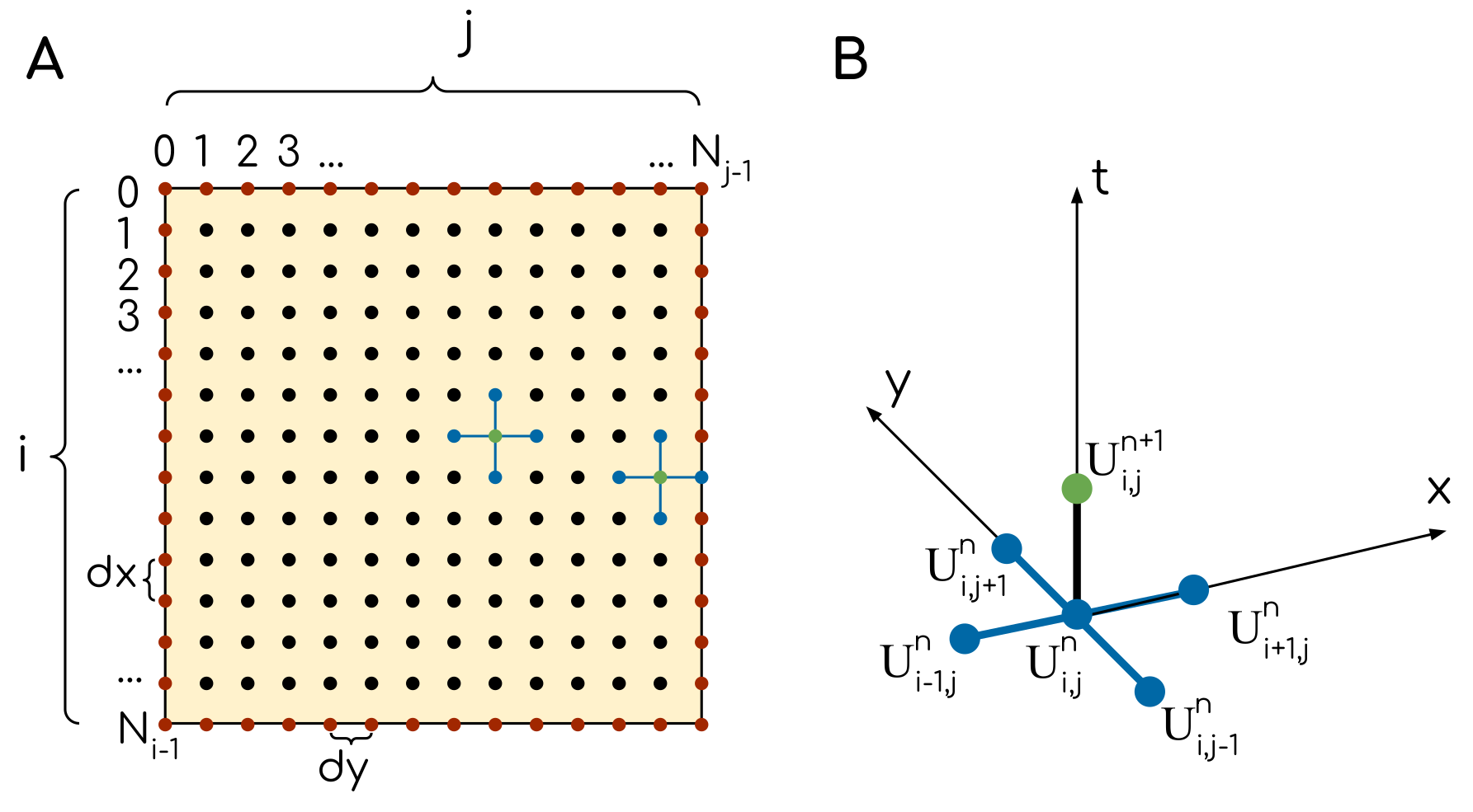
The grid (A) and the template (B) of the numerical scheme for the heat equation. Red dots indicate the grid nodes, where the values are taken from the boundary conditions. Black dots are internal grid nodes. The grid node in which the values is computes is shown in green. There are two examples of how the template (B) is applied to the grid (A).

With the grid defined, one can use the following explicit approximation for the differential equation:

\[\frac{U^{n+1}_{i,j}-U^{n}_{i,j}}{t_n}=a\left(\frac{U^n_{i-1,j}-2U^{n}_{i,j}+U^n_{i+1,j}}{dx} + \frac{U^n_{i,j-1}-2U^{n}_{i,j}+U^n_{i,j+1}}{dx}\right)\]

Here we used basic approximations for the first and second derivatives \(\frac{df}{dx}\approx\frac{f(x+dx)-f(x)}{dx}\) and \(\frac{d^2f}{dx^2}\approx\frac{f(x-dx)-2f(x)+f(x+dx)}{dx^2}\). In the equation above, the values on the next time step, \(U^{n+1}_{i,j}\) are unknown. Indeed, if \(n=0\), the only unknown value in equation for each \(i\) and \(j\) is \(U^1_{ij}\): the rest are determined by the initial condition. Going through all possible values of \(i\) and \(j\), one can compute the grid function \(U^n_{i,j}\) at \(n=1\). This procedure is then repeated for \(n=2\) and so on. Note that the values at the borders can not be computed from the equation above, since some of the required values will be out of the spatial region (e.g. \(U^n_{i-1,j}\) when \(i=0\)). This is where the boundary conditions are used.

The numerical scheme can then be rearranged to give an explicit expression for these values:

\[U^{n+1}_{i,j}= U^{n}_{i,j} + dh\cdot a\left(\frac{U^n_{i-1,j}-2U^{n}_{i,j}+U^n_{i+1,j}}{dx} + \frac{U^n_{i,j-1}-2U^{n}_{i,j}+U^n_{i,j+1}}{dx}\right)\]

And this is the expression we are going to use in our code.

The choice of the spatial steps \(dx\) and \(dy\) (or equally the choice of number of spatial steps \(N_x\) and \(N_y\)) are determined by the required spatial resolution. With the spatial steps set, the time step is limited by the stability of the numerical approximation of the equation, i.e. by:

\[dt \leq \frac{1}{2a}\frac{1}{\frac{1}{dx^2}+\frac{1}{dy^2}}=\frac{dx^2dy^2}{2a(dx^2+dy^2)}\]

We are going to be using the maximum possible time steps, as determined by the expression above.

Porting the code

Even though the problem is two-dimensional, we are still going to use one-dimensional arrays in CUDA. This allows for an explicit control of the memory access pattern. We want neighboring threads to access the neighboring elements of an array, so that the limited amounts of cache will be used efficiently. For that, we will use a helper function that computes the one-dimensional index from two indices:

getIndex(const int i, const int j, const int width)
{
    return i*width + j;
}

Here, width is a width of a two-dimensional array, i and j are the two-dimensional indices.

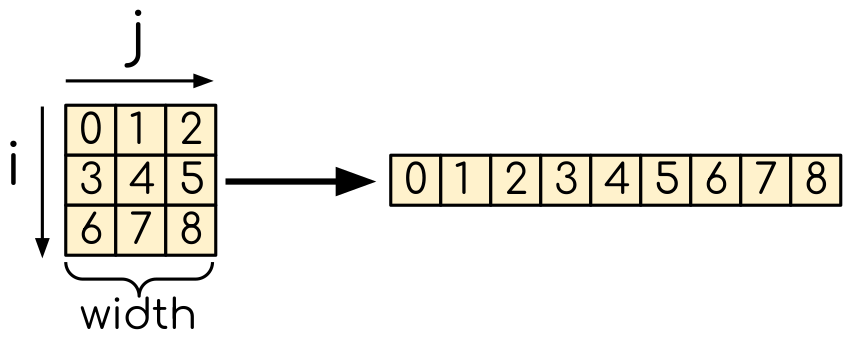
Mapping of the two-dimensional array into one-dimensional. The numbers represent the number of the element in 1D array.

Since we are going to use non-trivial data access pattern in the following examples, it is good idea to constantly check for errors. Not to overload the code with extra checks after every API call, we are going to use the following function from the CUDA API:

cudaGetLastError(..)

__host__​ __device__​ cudaError_t cudaGetLastError(void)

This function will check if there were any CUDA API errors in the previous calls and should return cudaSuccess if there were none. We will check this, and print an error message if this was not the case. In order to render a human-friendly string that describes an error, the cudaGetErrorString(..) function from the CUDA API will be used:

cudaGetErrorString(..)

__host__​ __device__ ​const char* cudaGetErrorString(cudaError_t error)

This will return a string, that we are going to print in case there were errors.

We will also need to use the getIndex(..) function from the device code. To do so, we will need to ask a compiler to compile it for the device execution. This is done by adding a __device__ specifier to its definition, will make the function available in the device code but not available in the host code. Since we are also using it when populating the initial conditions, we need a __host__ specifier for this function as well.

Initial CUDA port

C++CUDA (solution)

/*
 * Based on CSC materials from:
 * 
 * https://github.com/csc-training/openacc/tree/master/exercises/heat
 *
 */
#include <algorithm>
#include <stdio.h>
#include <stdlib.h>
#include <string.h>
#include <time.h>

#include "pngwriter.h"

/* Convert 2D index layout to unrolled 1D layout
 *
 * \param[in] i      Row index
 * \param[in] j      Column index
 * \param[in] width  The width of the area
 * 
 * \returns An index in the unrolled 1D array.
 */
int getIndex(const int i, const int j, const int width)
{
    return i*width + j;
}

int main()
{
    const int nx = 200;   // Width of the area
    const int ny = 200;   // Height of the area

    const float a = 0.5;     // Diffusion constant

    const float dx = 0.01;   // Horizontal grid spacing 
    const float dy = 0.01;   // Vertical grid spacing

    const float dx2 = dx*dx;
    const float dy2 = dy*dy;

    const float dt = dx2 * dy2 / (2.0 * a * (dx2 + dy2)); // Largest stable time step
    const int numSteps = 5000;                             // Number of time steps
    const int outputEvery = 1000;                          // How frequently to write output image

    int numElements = nx*ny;

    // Allocate two sets of data for current and next timesteps
    float* Un   = (float*)calloc(numElements, sizeof(float));
    float* Unp1 = (float*)calloc(numElements, sizeof(float));

    // Initializing the data with a pattern of disk of radius of 1/6 of the width
    float radius2 = (nx/6.0) * (nx/6.0);
    for (int i = 0; i < nx; i++)
    {
        for (int j = 0; j < ny; j++)
        {
            int index = getIndex(i, j, ny);
            // Distance of point i, j from the origin
            float ds2 = (i - nx/2) * (i - nx/2) + (j - ny/2)*(j - ny/2);
            if (ds2 < radius2)
            {
                Un[index] = 65.0;
            }
            else
            {
                Un[index] = 5.0;
            }
        }
    }

    // Fill in the data on the next step to ensure that the boundaries are identical.
    memcpy(Unp1, Un, numElements*sizeof(float));

    // Timing
    clock_t start = clock();

    // Main loop
    for (int n = 0; n <= numSteps; n++)
    {
        // Going through the entire area
        for (int i = 1; i < nx-1; i++)
        {
            for (int j = 1; j < ny-1; j++)
            {
                const int index = getIndex(i, j, ny);
                float uij = Un[index];
                float uim1j = Un[getIndex(i-1, j, ny)];
                float uijm1 = Un[getIndex(i, j-1, ny)];
                float uip1j = Un[getIndex(i+1, j, ny)];
                float uijp1 = Un[getIndex(i, j+1, ny)];

                // Explicit scheme
                Unp1[index] = uij + a * dt * ( (uim1j - 2.0*uij + uip1j)/dx2 + (uijm1 - 2.0*uij + uijp1)/dy2 );
            }
        }
        // Write the output if needed
        if (n % outputEvery == 0)
        {
            char filename[64];
            sprintf(filename, "heat_%04d.png", n);
            save_png(Un, nx, ny, filename, 'c');
        }
        // Swapping the pointers for the next timestep
        std::swap(Un, Unp1);
    }

    // Timing
    clock_t finish = clock();
    printf("It took %f seconds\n", (double)(finish - start) / CLOCKS_PER_SEC);

    // Release the memory
    free(Un);
    free(Unp1);
    
    return 0;
}

1. Change the extension to .cu, add device buffers, allocate memory.

2. Prepare kernel configuration parameters. Since we have a double loop over coordinates, it is convinient to map it to two-dimensional block of threads. Note that the total number of threads per block will be multiple of the number of threads in each dimensions, so it is easy to assign too many threads to a single block: this number is limited by 1024 for all NVidia GPUs. Decide the size of the block and compute the required number of blocks and create corresponding dim3 variables. It is convinient to use #define to specify the block sizes in each direction, since we are going to need them in the GPU code.

3. At the beginning of the main loop, copy data to the GPU.

4. Add a __device__ and __host__ specifiers to the getIndex(..) function definition.

   What will happen, if the __host__ __device__ function has the following line in its definition: printf("%ld\n", 13);?

   1. Nothing. Everything will compile and execute fine.

   2. The code will not compile — one can not use printf() in the device code.

   3. The code will compile with a warning, but will not execute.

   4. The code will compile with a warning and will execute printing number “13” many times.

   5. The code will compile with two warnings, but will not execute.

   6. The code will compile with two warnings, and will execute printing number “13” many times.

   Solution

   The added line should cause compiler to issue a warning. Since this line is in the __host__ __device__ function, there are going to be two warnings: one from the CPU compiler, one from the GPU compiler. All modern versions of CUDA allow printing from the kernels, althogh the order in which threads are printing is quite random.

4. Create a gpu kernel and move the double loop over coordinates into it. Change the loop indices to the components of the respective thread indices. Make sure that the data outside the domain is not accessed by installing a conditional on the indices (see the iteration limits of the original loops).

5. After the kernel is executed, copy the data back to the host memory.

Moving data ownership to the device

There is a lot of possibilities to improve the performance of in the current implementation. One of them is to reduce the number of the host-device and device-to host data transfers. Even though the transfers are relatively fast, they are much slower than accessing the memory in the kernel call. Eliminating the transfers is one of the most basic and most effitient improvements.

Note that in more complicated cases, eliminating the data transfers between host and device can be challenging. For instance, in cases where not all the computational procedures are ported to the GPU. This may happen on the early stages of the code porting, or because it is more effitient to compute some parts of the algorithm on a CPU. In this cases, effort should be made to hide the copy behind the computations: the compute kernels and copy calls use different resources. These two operations can be done simultaneously: while GPU is busy computing, the data can be copied on the background. One should also consider using CPU efficiently: if everything is computed on a device, host will be idling. This is a waste of resources. In some cases one can copy some data to the host memory, do the computations and copy data back while the device is still computing.

Removing unnessesary host to device and device to host data transfers, can also be looked at as the change in the data ownerhip. Now the device holds the data, do all computational procedures and, occasionally, the data is copied back to the CPU for e.g. output. This is exactly the case in our code: there is nothing to compute between two consequative time steps, so there is no need to copy data to the host on each step. The data only needed on the host for the output.

In the following exercise we will eliminate the unnessesary data transfers and will make the device responsible for holding current data.

Moving the data ownership to the device

CUDACUDA: device owns the data (solution)

/*
 * Based on CSC materials from:
 * 
 * https://github.com/csc-training/openacc/tree/master/exercises/heat
 *
 */
#include <algorithm>
#include <stdio.h>
#include <stdlib.h>
#include <string.h>
#include <time.h>

#include "pngwriter.h"

#define BLOCK_SIZE_X 16
#define BLOCK_SIZE_Y 16

/* Convert 2D index layout to unrolled 1D layout
 *
 * \param[in] i      Row index
 * \param[in] j      Column index
 * \param[in] width  The width of the area
 * 
 * \returns An index in the unrolled 1D array.
 */
int __host__ __device__ getIndex(const int i, const int j, const int width)
{
    return i*width + j;
}

__global__ void evolve_kernel(const float* Un, float* Unp1, const int nx, const int ny, const float dx2, const float dy2, const float aTimesDt)
{
    int i = threadIdx.x + blockIdx.x*blockDim.x;
    if (i > 0 && i < nx - 1)
    {
        int j = threadIdx.y + blockIdx.y*blockDim.y;
        if (j > 0 && j < ny - 1)
        {
            const int index = getIndex(i, j, ny);
            float uij = Un[index];
            float uim1j = Un[getIndex(i-1, j, ny)];
            float uijm1 = Un[getIndex(i, j-1, ny)];
            float uip1j = Un[getIndex(i+1, j, ny)];
            float uijp1 = Un[getIndex(i, j+1, ny)];

            // Explicit scheme
            Unp1[index] = uij + aTimesDt * ( (uim1j - 2.0*uij + uip1j)/dx2 + (uijm1 - 2.0*uij + uijp1)/dy2 );
        }
    }
}

int main()
{
    const int nx = 200;   // Width of the area
    const int ny = 200;   // Height of the area

    const float a = 0.5;     // Diffusion constant

    const float dx = 0.01;   // Horizontal grid spacing 
    const float dy = 0.01;   // Vertical grid spacing

    const float dx2 = dx*dx;
    const float dy2 = dy*dy;

    const float dt = dx2 * dy2 / (2.0 * a * (dx2 + dy2)); // Largest stable time step
    const int numSteps = 5000;                             // Number of time steps
    const int outputEvery = 1000;                          // How frequently to write output image

    int numElements = nx*ny;

    // Allocate two sets of data for current and next timesteps
    float* h_Un   = (float*)calloc(numElements, sizeof(float));
    float* h_Unp1 = (float*)calloc(numElements, sizeof(float));

    // Initializing the data with a pattern of disk of radius of 1/6 of the width
    float radius2 = (nx/6.0) * (nx/6.0);
    for (int i = 0; i < nx; i++)
    {
        for (int j = 0; j < ny; j++)
        {
            int index = getIndex(i, j, ny);
            // Distance of point i, j from the origin
            float ds2 = (i - nx/2) * (i - nx/2) + (j - ny/2)*(j - ny/2);
            if (ds2 < radius2)
            {
                h_Un[index] = 65.0;
            }
            else
            {
                h_Un[index] = 5.0;
            }
        }
    }

    // Fill in the data on the next step to ensure that the boundaries are identical.
    memcpy(h_Unp1, h_Un, numElements*sizeof(float));

    float* d_Un;
    float* d_Unp1;

    cudaMalloc((void**)&d_Un, numElements*sizeof(float));
    cudaMalloc((void**)&d_Unp1, numElements*sizeof(float));

    dim3 numBlocks(nx/BLOCK_SIZE_X + 1, ny/BLOCK_SIZE_Y + 1);
    dim3 threadsPerBlock(BLOCK_SIZE_X, BLOCK_SIZE_Y);

    // Timing
    clock_t start = clock();

    // Main loop
    for (int n = 0; n <= numSteps; n++)
    {
        cudaMemcpy(d_Un, h_Un, numElements*sizeof(float), cudaMemcpyHostToDevice);
        cudaMemcpy(d_Unp1, h_Unp1, numElements*sizeof(float), cudaMemcpyHostToDevice);

        evolve_kernel<<<numBlocks, threadsPerBlock>>>(d_Un, d_Unp1, nx, ny, dx2, dy2, a*dt);

        cudaMemcpy(h_Un, d_Un, numElements*sizeof(float), cudaMemcpyDeviceToHost);
        cudaMemcpy(h_Unp1, d_Unp1, numElements*sizeof(float), cudaMemcpyDeviceToHost);

        // Write the output if needed
        if (n % outputEvery == 0)
        {
            cudaError_t errorCode = cudaGetLastError();
            if (errorCode != cudaSuccess)
            {
                printf("Cuda error %d: %s\n", errorCode, cudaGetErrorString(errorCode));
                exit(0);
            }
            char filename[64];
            sprintf(filename, "heat_%04d.png", n);
            save_png(h_Un, nx, ny, filename, 'c');
        }
        // Swapping the pointers for the next timestep
        std::swap(h_Un, h_Unp1);
    }

    // Timing
    clock_t finish = clock();
    printf("It took %f seconds\n", (double)(finish - start) / CLOCKS_PER_SEC);

    // Release the memory
    free(h_Un);
    free(h_Unp1);

    cudaFree(d_Un);
    cudaFree(d_Unp1);
    
    return 0;
}

1. Use the solution of the previous example as a starting point.

2. Move the host to device copy calls to before the main loop (i.e. before the loop over the time steps).

3. Move the device to host copy into the conditional on the output. Only the current layer of data is needed (Un).

4. Change the pointer swapping from the host pointers to the device pointer. In CUDA, the device buffers are just pointers, so the usual operations work the same way as with the host pointer.

5. Now, the Unp1 array on the host can be removed, since it is redundant.`

Using shared memory

Another useful way to optimize the device code is to reduce the number of global memory calls in the GPU kernel. Even though the memory bandwith is very high on modern GPUs, many threads are using it. And there is not so much cache to go with either. Minimizing the calls to the global memory can drastically improve the computational efficiency of the application. Shared memory is the cache memory that is shared between threads in a block. The access pattern in our GPU kernel is such that neighboring threads aggess neighboring data. This means that some of the data is accessed by neighboring threads. In fact, each value of the grid function, \(U^n_{ij}\) is read 5 times — once as the central point in the thread (i,j) and once as a side point in threads (i-1,j), (i+1,j), (i,j-1) and (i,j+1). What can be done instead is, at the beginning of the kernel call, we read the value of the central point into the shared memory. Than, we ask all the threads to wait until all the values are read. Once the data is ready, we proceed with the computation. Additionally, one will hate to take care of the extra values at the borders of the thread block, which we will see while working on the example.

But before we start, we need to learn the extra tools that we are going to need. There are two ways of allocating the shared memory: dynamic and static. The dynamic allocation is needed if the size of the required shared memory is not known at the compilation time. In our case, we know exactly how much space is needed, so we will be using static alocation. To allocate the shared memory of size N, one needs to add in the GPU kernel:

__shared__ float s_x[N];

The __shared__ modifier will tell the compiler that this array should be allocated in the shared memory space. Note that we used the s_ prefix to the array. This is not necessary, but helps for the code transparency.

We will also need to make sure that all threads in the block are done reading data and placing it into the shared memory. This can be done with the call to __syncthreads(..) function inside the GPU kernel:

__syncthreads(..)

void __syncthreads()

Calling this function will block all the threads from execution until they reach the point where this function call is made. Note that __syncthreads(..) should be called unconditionally, from all threads in the thread block, so that this point in code can be reached by all the threads.

In the following example, we will change the GPU kernel to use the shared memory to hold all the values needed for the current computational time step.

Use shared memory

CUDA: device owns the dataCUDA: use shared memory (solution)

/*
 * Based on CSC materials from:
 * 
 * https://github.com/csc-training/openacc/tree/master/exercises/heat
 *
 */
#include <algorithm>
#include <stdio.h>
#include <stdlib.h>
#include <string.h>
#include <time.h>

#include "pngwriter.h"

#define BLOCK_SIZE_X 16
#define BLOCK_SIZE_Y 16

/* Convert 2D index layout to unrolled 1D layout
 *
 * \param[in] i      Row index
 * \param[in] j      Column index
 * \param[in] width  The width of the area
 * 
 * \returns An index in the unrolled 1D array.
 */
int __host__ __device__ getIndex(const int i, const int j, const int width)
{
    return i*width + j;
}

__global__ void evolve_kernel(const float* Un, float* Unp1, const int nx, const int ny, const float dx2, const float dy2, const float aTimesDt)
{
    int i = threadIdx.x + blockIdx.x*blockDim.x;
    if (i > 0 && i < nx - 1)
    {
        int j = threadIdx.y + blockIdx.y*blockDim.y;
        if (j > 0 && j < ny - 1)
        {
            const int index = getIndex(i, j, ny);
            float uij = Un[index];
            float uim1j = Un[getIndex(i-1, j, ny)];
            float uijm1 = Un[getIndex(i, j-1, ny)];
            float uip1j = Un[getIndex(i+1, j, ny)];
            float uijp1 = Un[getIndex(i, j+1, ny)];

            // Explicit scheme
            Unp1[index] = uij + aTimesDt * ( (uim1j - 2.0*uij + uip1j)/dx2 + (uijm1 - 2.0*uij + uijp1)/dy2 );
        }
    }
}

int main()
{
    const int nx = 200;   // Width of the area
    const int ny = 200;   // Height of the area

    const float a = 0.5;     // Diffusion constant

    const float dx = 0.01;   // Horizontal grid spacing 
    const float dy = 0.01;   // Vertical grid spacing

    const float dx2 = dx*dx;
    const float dy2 = dy*dy;

    const float dt = dx2 * dy2 / (2.0 * a * (dx2 + dy2)); // Largest stable time step
    const int numSteps = 5000;                             // Number of time steps
    const int outputEvery = 1000;                          // How frequently to write output image

    int numElements = nx*ny;

    // Allocate two sets of data for current and next timesteps
    float* h_Un   = (float*)calloc(numElements, sizeof(float));

    // Initializing the data with a pattern of disk of radius of 1/6 of the width
    float radius2 = (nx/6.0) * (nx/6.0);
    for (int i = 0; i < nx; i++)
    {
        for (int j = 0; j < ny; j++)
        {
            int index = getIndex(i, j, ny);
            // Distance of point i, j from the origin
            float ds2 = (i - nx/2) * (i - nx/2) + (j - ny/2)*(j - ny/2);
            if (ds2 < radius2)
            {
                h_Un[index] = 65.0;
            }
            else
            {
                h_Un[index] = 5.0;
            }
        }
    }

    float* d_Un;
    float* d_Unp1;

    cudaMalloc((void**)&d_Un, numElements*sizeof(float));
    cudaMalloc((void**)&d_Unp1, numElements*sizeof(float));

    cudaMemcpy(d_Un, h_Un, numElements*sizeof(float), cudaMemcpyHostToDevice);
    cudaMemcpy(d_Unp1, h_Un, numElements*sizeof(float), cudaMemcpyHostToDevice);

    dim3 numBlocks(nx/BLOCK_SIZE_X + 1, ny/BLOCK_SIZE_Y + 1);
    dim3 threadsPerBlock(BLOCK_SIZE_X, BLOCK_SIZE_Y);

    // Timing
    clock_t start = clock();

    // Main loop
    for (int n = 0; n <= numSteps; n++)
    {
        evolve_kernel<<<numBlocks, threadsPerBlock>>>(d_Un, d_Unp1, nx, ny, dx2, dy2, a*dt);

        // Write the output if needed
        if (n % outputEvery == 0)
        {
            cudaMemcpy(h_Un, d_Un, numElements*sizeof(float), cudaMemcpyDeviceToHost);
            cudaError_t errorCode = cudaGetLastError();
            if (errorCode != cudaSuccess)
            {
                printf("Cuda error %d: %s\n", errorCode, cudaGetErrorString(errorCode));
                exit(0);
            }
            char filename[64];
            sprintf(filename, "heat_%04d.png", n);
            save_png(h_Un, nx, ny, filename, 'c');
        }

        std::swap(d_Un, d_Unp1);
    }

    // Timing
    clock_t finish = clock();
    printf("It took %f seconds\n", (double)(finish - start) / CLOCKS_PER_SEC);

    // Release the memory
    free(h_Un);

    cudaFree(d_Un);
    cudaFree(d_Unp1);
    
    return 0;
}

1. Use the previous version of the code as a starting point.

2. Define the __shared__ array in the device kernel. The size should be big enough to accomodate the central points for the block, plus the two elements for each dimension — one at each border.

3. Fill in all the central elements of the array by using all the threads in the block.

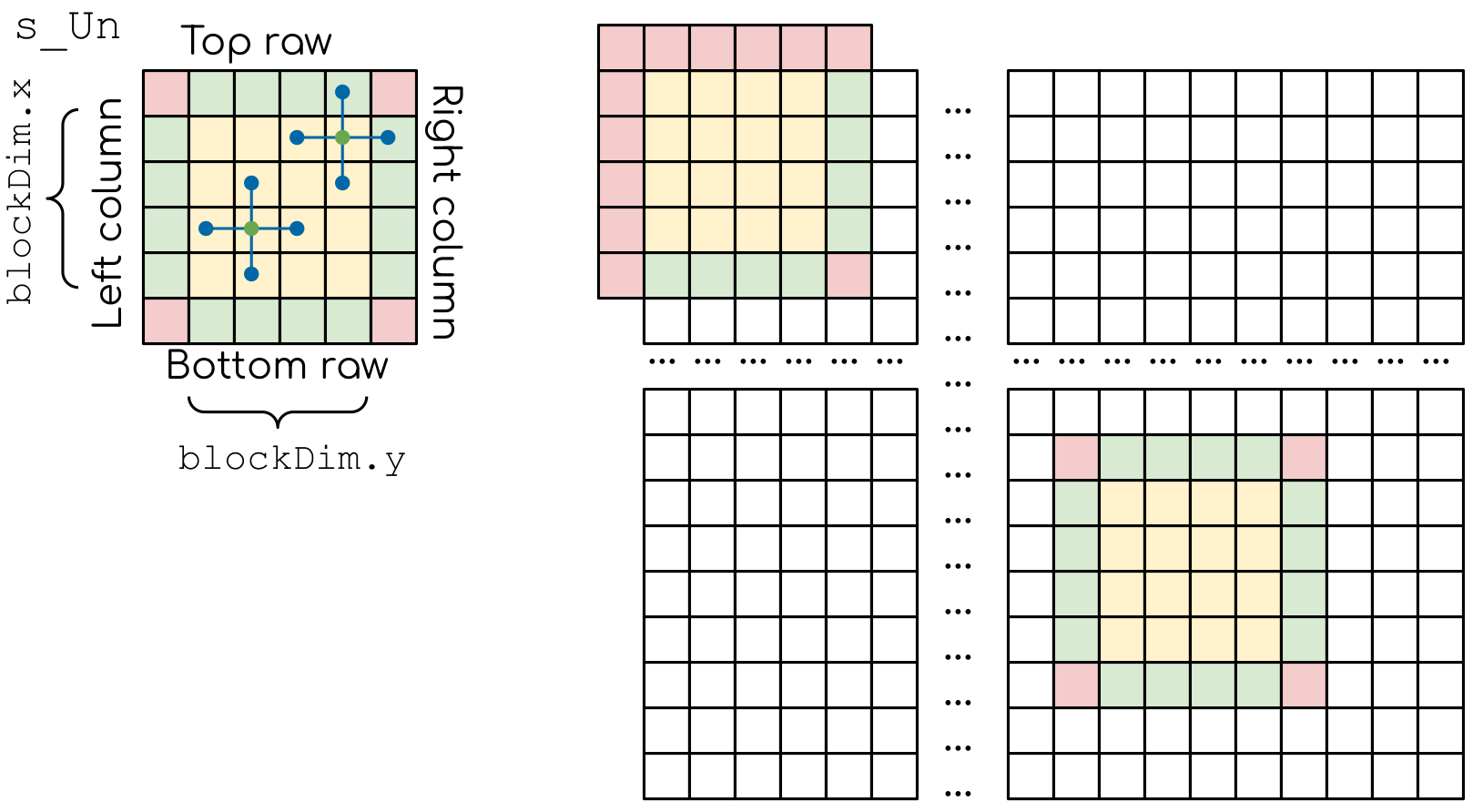
The shared memory array s_Un, and how it maps to the global thread grid. In addition to the central region (yellow), the shared memory adday should contain the border elements (green), so that we can compute all the values of the function Un on the next time step. In the boder blocks the border elements are not populated because the values of the function there are taken from the boundary conditions. Note that trying to populate these region will lead to adressing memory outside the allocated array, so proper conditionals have to be added to avoid segmentation fault errors.

4. Use the threads that are next to the border of the block to fill the bordering parts of the array. Make sure that you are not accessing the data outside the allocated global memory array.

5. Add blocking syncronization with __syncthreads(..) after all the data is read.

6. Change the compute part to use the shared memory instead of the global memory.