GPU programming

Questions

• What are the high-level and low-level methods for GPU programming in Julia?

• How do GPU Arrays work?

• How are GPU kernels written?

Instructor note

• 30 min teaching

• 40 min exercises

Julia has first-class support for GPU programming through the following packages that target GPUs from all major vendors:

• CUDA.jl for NVIDIA GPUs

• AMDGPU.jl for AMD GPUs

• oneAPI.jl for Intel GPUs

• Metal.jl for Apple M-series GPUs

CUDA.jl is the most mature, AMDGPU.jl is somewhat behind but still ready for general use, while oneAPI.jl and Metal.jl are functional but might contain bugs, miss some features and provide suboptimal performance.

NVIDIA still dominates the HPC accelerator market, but AMD has recently made big strides in this sector and both Frontier and LUMI (ranked 1st and 3rd on the Top500 list in June 2023) are built on AMD GPUs. This section will show code examples targeting all four frameworks, but for certain functionalities only the CUDA.jl version will be shown.

CUDA.jl, AMDGPU.jl, oneAPI.jl and Metal.jl offer both user-friendly high-level abstractions that require very little programming effort and a lower level approach for writing kernels for fine-grained control.

Setup

NVIDIAAMDIntelApple

Installing CUDA.jl:

using Pkg
Pkg.add("CUDA")

To use the Julia GPU stack, one needs to have the relevant GPU drivers and programming toolkits installed. GPU drivers are already installed on HPC systems while on your own machine you will need to install them yourself (see e.g. these instructions from NVIDIA). Programming toolkits for CUDA can be installed automatically through Julia’s artifact system upon the first usage:

NVIDIAAMDIntelApple

Installing CUDA toolkit:

using CUDA
CUDA.versioninfo()

Access to GPUs

To fully experience the walkthrough in this episode we need to have access to a GPU device and the necessary software stack.

• Access to a HPC system with GPUs and a Julia installation is optimal.

• If you have a powerful GPU on your own machine you can also install the drivers and toolkits yourself. Another option is to use

• JuliaHub, a commercial cloud platform from Julia Computing with access to Julia’s ecosystem of packages and GPU hardware.

• Or one can use Google Colab which requires a Google account and a manual Julia installation, but using simple NVIDIA GPUs is free. Google Colab does not support Julia, but a helpful person on the internet has created a Colab notebook that can be reused for Julia computing on Colab.

GPUs vs CPUs

We first briefly discuss the hardware differences between GPUs and CPUs. This will help us understand the rationale behind the GPU programming methods described later.

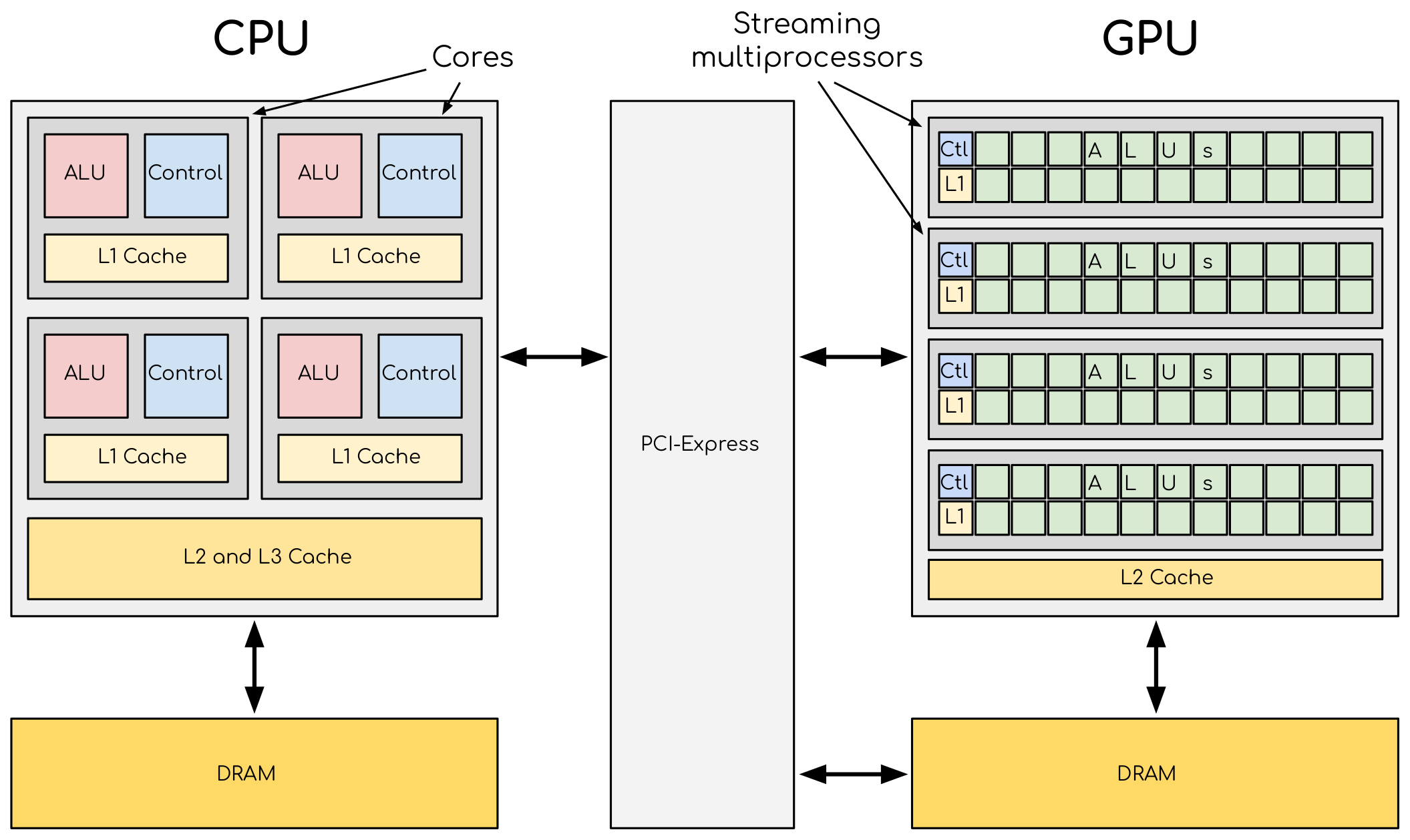
A comparison of CPU and GPU architectures. A CPU has a complex core structure and packs several cores on a single chip. GPU cores are very simple in comparison and they share data, allowing to pack more cores on a single chip.

Some key aspects of GPUs that need to be kept in mind:

• The large number of compute elements on a GPU (in the thousands) can enable extreme scaling for data parallel tasks (single-program multiple-data, SPMD)

• GPUs have their own memory. This means that data needs to be transferred to and from the GPU during the execution of a program.

• Cores in a GPU are arranged into a particular structure. At the highest level they are divided into “streaming multiprocessors” (SMs). Some of these details are important when writing own GPU kernels.

The array interface

GPU programming with Julia can be as simple as using a different array type instead of regular Base.Array arrays:

• CuArray from CUDA.jl for NVIDIA GPUs

• ROCArray from AMDGPU.jl for AMD GPUs

• oneArray from oneAPI.jl for Intel GPUs

• MtlArray from Metal.jl for Apple GPUs

These array types closely resemble Base.Array which enables us to write generic code which works on both types.

The following code copies an array to the GPU and executes a simple operation on the GPU:

NVIDIAAMDIntelApple

using CUDA

A_d = CuArray([1,2,3,4])
A_d .+= 1

Moving an array back from the GPU to the CPU is simple:

A = Array(A_d)

However, the overhead of copying data to the GPU makes such simple calculations very slow.

Let’s have a look at a more realistic example: matrix multiplication. We create two random arrays, one on the CPU and one on the GPU, and compare the performance:

NVIDIAAMDIntelApple

using BenchmarkTools
using CUDA

A = rand(2^9, 2^9);
A_d = CuArray(A);

@btime $A * $A;
# need to synchronize to let the CPU wait for the GPU kernel to finish
@btime CUDA.@sync $A_d * $A_d;

There should be a considerable speedup!

Effect of array size

Does the size of the array affect how much the performance improves?

Solution

For example, on an Mi250X AMD GPU:

using AMDGPU
using BenchmarkTools

A = rand(2^9, 2^9); A_d = ROCArray(A);

# 1 CPU core:
@btime $A * $A;
# 5.472 ms (2 allocations: 2.00 MiB)
# 64 CPU cores:
@btime $A * $A;
# 517.722 μs (2 allocations: 2.00 MiB)
# GPU
@btime begin
    $A_d * $A_d;
end
# 115.805 μs (21 allocations: 1.06 KiB)

# ~47 times faster than 1 CPU core, ~5 times faster than 64 cores

A = rand(2^10, 2^10); A_d = ROCArray(A);

# 1 CPU core
@btime $A * $A;
# 43.364 ms (2 allocations: 8.00 MiB)
# 64 CPU cores
@btime $A*$A;
# 2.929 ms (2 allocations: 8.00 MiB)
@btime begin
   $A_d * $A_d;
   AMDGPU.synchronize()
end
# 173.316 μs (21 allocations: 1.06 KiB)

# ~250 times faster than one CPU core, ~17 times faster than 64 cores

A = rand(2^11, 2^11); A_d = ROCArray(A);

# 1 CPU core
@btime $A * $A;
# 344.364 ms (2 allocations: 32.00 MiB)
# 64 CPU cores
@btime $A * $A;
# 30.081 ms (2 allocations: 32.00 MiB)
@btime begin
    $A_d * $A_d;
end
# 866.348 μs (21 allocations: 1.06 KiB)

# ~400 times faster than 1 core, 35 times faster than 64 cores

A = rand(2^12, 2^12); A_d = ROCArray(A);

# 1 CPU core
@btime $A*$A;
# 3.221 s (2 allocations: 128.00 MiB)
# 64 CPU cores
@btime $A*$A;
# 159.563 ms (2 allocations: 128.00 MiB)
# GPU
@btime begin
   $A_d * $A_d;
   AMDGPU.synchronize()
end
# 5.910 ms (21 allocations: 1.06 KiB)

# ~550 times faster than 1 CPU core, 27 times faster than 64 CPU cores

Vendor libraries

Support for using GPU vendor libraries from Julia is currently only supported on NVIDIA GPUs. NVIDIA libraries contain precompiled kernels for common operations like matrix multiplication (cuBLAS), fast Fourier transforms (cuFFT), linear solvers (cuSOLVER), etc. These kernels are wrapped in CUDA.jl and can be used directly with CuArrays:

# create a 100x100 Float32 random array and an uninitialized array
A = CUDA.rand(2^9, 2^9);
B = CuArray{Float32, 2}(undef, 2^9, 2^9);

# regular matrix multiplication uses cuBLAS under the hood
A * A

# use LinearAlgebra for matrix multiplication
using LinearAlgebra
mul!(B, A, A)

# use cuSOLVER for QR factorization
qr(A)

# solve equation A*X == B
A \ B

# use cuFFT for FFT
using CUDA.CUFFT
fft(A)

Convert from Base.Array or use GPU methods?

What is the difference between creating a random array in the following two ways?

Converting from Base.Arrayrand() method from CUDA.jl/AMDGPU.jl

A = rand(2^9, 2^9);
A_d = CuArray(A); # ROCArray(A) for AMDGPU

Solution

NVIDIAAMD

A = rand(2^9, 2^9);
A_d = CuArray(A);
typeof(A_d)
# CuArray{Float64, 2, CUDA.Mem.DeviceBuffer}

B_d = CUDA.rand(2^9, 2^9);
typeof(B_d)
# CuArray{Float32, 2, CUDA.Mem.DeviceBuffer}

The rand() method defined in CUDA.jl/AMDGPU.jl creates 32-bit floating point numbers while converting from a 64-bit float Base.Array to a CuArray/ROCArray retains it as Float64!

GPUs normally perform significantly better for 32-bit floats.

Higher-order abstractions

A powerful way to program GPUs with arrays is through Julia’s higher-order array abstractions. The simple element-wise addition we saw above, a .+= 1, is an example of this, but more general constructs can be created with broadcast, map, reduce, accumulate etc:

broadcastmapreduceaccumulate

broadcast(A_d) do x
    x += 1
end

Writing your own kernels

Not all algorithms can be made to work with the higher-level abstractions in CUDA.jl / AMDGPU.jl / oneAPI.jl / Metal.jl. In such cases it’s necessary to explicitly write our own GPU kernel.

Let’s take a simple example, adding two vectors:

function vadd!(C, A, B)
    for i in 1:length(A)
        @inbounds C[i] = A[i] + B[i]
    end
end

A = zeros(10) .+ 5.0;
B = ones(10);
C = similar(B);
vadd!(C, A, B)

We can already run this on the GPU with the @cuda (NVIDIA) or @roc (AMD) macro, which will compile vadd!() into a GPU kernel and launch it:

NVIDIAAMDIntelApple

A_d = CuArray(A);
B_d = CuArray(B);
C_d = similar(B_d);

@cuda vadd!(C_d, A_d, B_d)

But the performance would be terrible because each thread on the GPU would be performing the same loop! So we have to remove the loop over all elements and instead use the special threadIdx and blockDim functions, analogous respectively to threadid and nthreads for multithreading.

We can split work between the GPU threads by using a special function which returns the index of the GPU thread which executes it (e.g. threadIdx().x for NVIDIA and workitemIdx().x for AMD):

NVIDIAAMDIntelApple

function vadd!(C, A, B)
    index = threadIdx().x   # linear indexing, so only use `x`
    @inbounds C[index] = A[index] + B[index]
    return
end

A, B = CUDA.ones(2^9)*2, CUDA.ones(2^9)*3;
C = similar(A);

N = length(A)
@cuda threads=N vadd!(C, A, B)

@assert all(Array(C) .== 5.0)

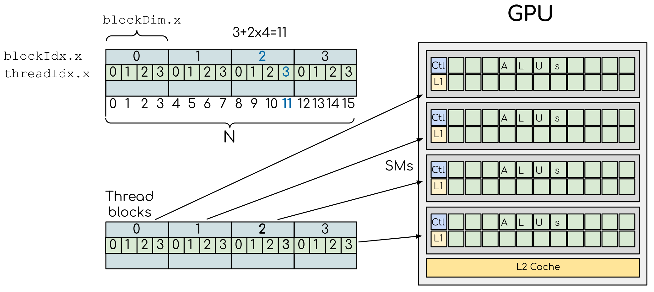
However, this implementation will not scale up to arrays that are larger than the maximum number of threads in a block! We can find out how many threads are supported on the GPU we are using:

NVIDIAAMDIntelApple

CUDA.attribute(device(), CUDA.DEVICE_ATTRIBUTE_MAX_THREADS_PER_BLOCK)

Clearly, GPUs have a limited number of threads they can run on a single SM. To parallelise over multiple SMs we need to run a kernel with multiple blocks where we also take advantage of the blockDim() and blockIdx() functions (in the case of NVIDIA):

NVIDIAAMDIntelApple

function vadd!(C, A, B)
    i = threadIdx().x + (blockIdx().x - 1) * blockDim().x
    if i <= length(A)
        @inbounds C[i] = A[i] + B[i]
    end
    return
end

A, B = ROCArray(ones(2^9)*2), ROCArray(ones(2^9)*3);
C = similar(A);

nthreads = 256
# smallest integer larger than or equal to length(A)/threads
numblocks = cld(length(A), nthreads)

# run using 256 threads
@cuda threads=nthreads blocks=numblocks vadd!(C, A, B)

@assert all(Array(C) .== 5.0)

We have been using 256 GPU threads, but this might not be optimal. The more threads we use the better is the performance, but the maximum number depends both on the GPU and the nature of the kernel.

To optimize the number of threads, we can first create the kernel without launching it, query it for the number of threads supported, and then launch the compiled kernel:

NVIDIAAMDIntelApple

# compile kernel
kernel = @cuda launch=false vadd!(C, A, B)
# extract configuration via occupancy API
config = launch_configuration(kernel.fun)
# number of threads should not exceed size of array
threads = min(length(A), config.threads)
# smallest integer larger than or equal to length(A)/threads
blocks = cld(length(A), threads)

# launch kernel with specific configuration
kernel(C, A, B; threads, blocks)

Restrictions in kernel programming

Within kernels, most of the Julia language is supported with the exception of functionality that requires the Julia runtime library. This means one cannot allocate memory or perform dynamic function calls, both of which are easy to do accidentally!

1D, 2D and 3D

CUDA.jl and AMDGPU.jl support indexing in up to 3 dimensions (x, y and z, e.g. threadIdx().x and workitemIdx().x). This is convenient for multidimensional data where thread blocks can be organised into 1D, 2D or 3D arrays of threads.

Debugging

Many things can go wrong with GPU kernel programming and unfortunately error messages are sometimes not very useful because of how the GPU compiler works.

Conventional print-debugging is often a reasonably effective way to debug GPU code. CUDA.jl provides macros that facilitate this:

• @cushow (like @show): visualize an expression and its result, and return that value.

• @cuprintln (like println): to print text and values.

• @cuaassert (like @assert) can also be useful to find issues and abort execution.

GPU code introspection macros also exist, like @device_code_warntype, to track down type instabilities.

More information on debugging can be found in the documentation.

Profiling

We can not use the regular Julia profilers to profile GPU code. However, for NVIDIA GPUs we can use the Nsight systems profiler simply by starting Julia like this:

$ nsys launch julia

To then profile a particular function, we prefix by the CUDA.@profile macro:

using CUDA
A = CuArray(zeros(10) .+ 5.0)
B = CuArray(ones(10))
C = CuArray(similar(B))
# first run it once to force compilation
@cuda threads=length(A) vadd!(C, A, B)
CUDA.@profile @cuda threads=length(A) vadd!(C, A, B)

When we quit the REPL again, the profiler process will print information about the executed kernels and API calls into report files. These can be inspected in a GUI, but summary statistics can also be printed in the terminal:

$ nsys stats report.nsys-rep

More information on profiling with NVIDIA tools can be found in the documentation.

For profiling Julia code running on AMD GPUs one can use rocprof - see the documentation.

Conditional use

Using functionality from CUDA.jl (or another GPU package) will result in a run-time error on systems without CUDA and a GPU. If GPU is required for a code to run, one can use an assertion:

using CUDA
@assert CUDA.functional(true)

However, it can be desirable to be able to write code that works systems both with and without GPUs. If GPU is optional, you can write a function to copy arrays to the GPU if one is present:

if CUDA.functional()
    to_gpu_or_not_to_gpu(x::AbstractArray) = CuArray(x)
else
    to_gpu_or_not_to_gpu(x::AbstractArray) = x
end

Some caveats apply and other solutions exist to address them as outlined in the documentation.

Exercises

Port sqrt_sum() to GPU

Try to GPU-port the sqrt_sum function we saw in an earlier episode:

function sqrt_sum(A)
    s = zero(eltype(A))
    for i in eachindex(A)
        @inbounds s += sqrt(A[i])
    end
    return s
end

• Use higher-order array abstractions to compute the sqrt-sum operation on a GPU!

• If you’re interested in how the performance changes, benchmark the CPU and GPU versions with @btime

Hint: You can do it on a single line…

Solution

First the square root should be taken of each element of the array, which we can do with map(sqrt,A). Next we perform a reduction with the + operator. Combining these steps:

A = CuArray([1 2 3; 4 5 6; 7 8 9])

reduce(+, map(sqrt,A))

GPU porting complete!

To benchmark:

A=ones(1024,1024);
A_d = CuArray(A);

# benchmark CPU function
@btime sqrt_sum($A)
#  2.664 ms (1 allocation: 16 bytes)

# benchmark also broadcast operations on the CPU:
@btime reduce(+, map(sqrt,$A))
#  2.930 ms (4 allocations: 8.00 MiB)
#  Slightly slower than the sqrt_sum function call but much larger memory allocations!

# benchmark GPU broadcast (result is from NVIDIA A100):
@btime reduce(+, map(sqrt, $A_d))
#  59.719 μs (119 allocations: 6.36 KiB)

Does LinearAlgebra provide acceleration?

Compare how long it takes to run a normal matrix multiplication and using the mul!() method from LinearAlgebra. Is there a speedup from using mul!()?

Solution

NVIDIAAMD

using CUDA, BenchmarkTools, LinearAlgebra

A = CUDA.rand(2^5, 2^5)
B = similar(A)
@btime $A*$A;
#  8.803 μs (16 allocations: 384 bytes)
@btime mul!($B, $A, $A);
#  7.282 μs (12 allocations: 224 bytes)

A = CUDA.rand(2^12, 2^12)
B = similar(A)
@btime $A*$A;
#  12.760 μs (28 allocations: 576 bytes)
@btime mul!($B, $A, $A)
#  11.020 μs (24 allocations: 416 bytes)

LinearAlgebra.mul!() is around 15-20% faster!

Compare broadcasting to kernel

Consider the vector addition function from above:

function vadd!(c, a, b)
    for i in 1:length(a)
        @inbounds c[i] = a[i] + b[i]
    end
end

• Write a kernel (or use the one shown above) and benchmark it with a moderately large vector.

• Then benchmark a broadcasted version of the vector addition. How does it compare to the kernel?

Solution

First define the kernel (for NVIDIA):

function vadd!(C, A, B)
    i = threadIdx().x + (blockIdx().x - 1) * blockDim().x
    if i <= length(A)
        @inbounds C[i] = A[i] + B[i]
    end
    return nothing
end

Define largish vectors:

A = CuArray(ones(2^20))
B = CuArray(ones(2^20).*2)
C = CuArray(similar(A))

Set nthreads and numblocks and benchmark kernel:

@btime $C .= $A .+ $B
nthreads = 1024
numblocks = cld(length(A), nthreads)

@btime CUDA.@sync @cuda threads=nthreads blocks=numblocks vadd!($C, $A, $B)
#  18.410 μs (33 allocations: 1.67 KiB)

Finally compare to the higher-level array interface:

@btime $C .= $A .+ $B
#  5.014 μs (27 allocations: 1.66 KiB)

The high-level abstraction is significantly faster!

Port Laplace function to GPU

Write a kernel for the lap2d! function!

Start with the regular version with @inbounds added:

function lap2d!(u, unew)
    M, N = size(u)
    for j in 2:N-1
        for i in 2:M-1
            @inbounds unew[i,j] = 0.25 * (u[i+1,j] + u[i-1,j] + u[i,j+1] + u[i,j-1])
        end
    end
end

Now start implementing a GPU kernel version.

1. The kernel function needs to end with return or return nothing.

2. The arrays are two-dimensional, so you will need both the .x and .y parts of threadIdx(), blockDim() and blockIdx().

3. You also need to specify tuples for the number of threads and blocks in the x and y dimensions, e.g. threads = (32, 32) and similarly for blocks (using cld).

   • Note the hardware limitations: the product of x and y threads cannot exceed it!

4. For debugging, you can print from inside a kernel using @cuprintln (e.g. to print thread numbers). But printing is slow so use small matrix sizes! It will only print during the first execution - redefine the function again to print again. If you get warnings or errors relating to types, you can use the code introspection macro @device_code_warntype to see the types inferred by the compiler.

5. Check correctness of your results! To test that the CPU and GPU versions give (approximately) the same results, for example:

   M = 4096
   N = 4096
   u = zeros(M, N);
   # set boundary conditions
   u[1,:] = u[end,:] = u[:,1] = u[:,end] .= 10.0;
   unew = copy(u);
   
   # copy to GPU and convert to Float32
   u_d, unew_d = CuArray(cu(u)), CuArray(cu(unew))
   
   for i in 1:1000
       lap2d!(u, unew)
       u = copy(unew)
   end
   
   for i in 1:1000
       @cuda threads=(nthreads, nthreads) blocks=(numblocks, numblocks) lap2d!(u_d, unew_d)
       u_d = copy(unew_d)
   end
   
   all(u .≈ Array(u_d))
   

6. Perform some benchmarking of the CPU and GPU methods of the function for arrays of various sizes and with different choices of nthreads. You will need to prefix the kernel execution with the CUDA.@sync macro to let the CPU wait for the GPU kernel to finish (otherwise you would be measuring the time it takes to only launch the kernel):

Solution

This is one possible GPU kernel version of lap2d!:

function lap2d_gpu!(u, unew)
    M, N = size(u)
    i = (blockIdx().x - 1) * blockDim().x + threadIdx().x
    j = (blockIdx().y - 1) * blockDim().y + threadIdx().y
    #@cuprintln("threads $i $j") #only for debugging!
    if i > 1 && j > 1 && i < M && j < N
        @inbounds unew[i,j] = 0.25 * (u[i+1,j] + u[i-1,j] + u[i,j+1] + u[i,j-1])
    end
    return nothing
end

To test it:

# set number of threads and blocks
nthreads = (16, 16)
numblocks = (cld(size(u, 1), nthreads[1]), cld(size(u, 2), nthreads[2]))

for i in 1:1000
   # call cpu and gpu versions
   lap2d!(u, unew)
   u = copy(unew)

   @cuda threads=nthreads blocks=numblocks lap2d_gpu!(u_d, unew_d)
   u_d = copy(unew_d)
end

# element-wise comparison
all(u .≈ Array(u_d))

To benchmark:

using BenchmarkTools
@btime lap2d!($u, $unew)
@btime CUDA.@sync @cuda threads=$nthreads blocks=$numblocks lap2d_gpu!($u_d, $unew_d)

See also

• JuliaGPU organisation

• CUDA.jl documentation

• AMDGPU.jl documentation

• JuliaCon2021 GPU workshop

• Advanced GPU programming tutorials