Writing performant Julia code

Questions

How should performance be measured?
How can I profile my Julia code?
Are there any performance pitfalls in Julia?

Instructor note

30 min teaching
20 min exercises

Introducing a toy example

As an example numerical problem, we will consider the discretized Laplace operator which is used widely in applications including numerical analysis, many physical problems, image processing and even machine learning. Here we will consider a simple two-dimensional implementation with a finite-difference formula, which reads:

\[u_{out}(i,j) = 0.25 [u(i−1,j) + u(i+1,j) + u(i,j−1) + u(i,j+1)]\]

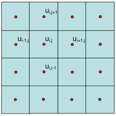
../_images/2D-Laplace-operator.png — An example of the discretization of the 2D Laplace operator.

In Julia, this can be implemented as:

function lap2d!(u, unew)
    M, N = size(u)
    for j in 2:N-1
        for i in 2:M-1
            unew[i,j] = 0.25 * (u[i+1,j] + u[i-1,j] + u[i,j+1] + u[i,j-1])
        end 
    end
end

Note that we follow the Julia convention of appending an exclamation mark to functions that mutate their arguments.

We now start by initializing the two 64-bit floating point arrays \(u\) and \(unew\), and arbitrarily set the boundaries to 10.0 to have something interesting to simulate:

function setup(N=4096, M=4096)
    u = zeros(M, N)
    # set boundary conditions
    u[1,:] = u[end,:] = u[:,1] = u[:,end] .= 10.0
    unew = copy(u);
    return u, unew
end

To simulate something that resembles e.g. the evolution of temperature in a 2D heat conductor (although we’ve completely ignored physical constants and time-stepping involved in solving the heat equation), we could run a loop of say 1000 “time” steps and visualize the results with the heatmap method of the Plots package:

u, unew = setup()

for i in 1:1000
    lap2d!(u, unew)
    # copy new computed field to old array
    u = copy(unew)
    # you can using the following expression if you get a warning "Assignment to `u` in soft scope is ambiguous because ..."
    # global u = copy(unew)
end

using Plots
heatmap(u)

Benchmarking

Base Julia already has the @time macro to print the time it takes to execute an expression. However, to get more accurate values it is better to rely on the BenchmarkTools.jl framework, which provides convenient macros to perform benchmarking:

@btime: for quick sanity checks, prints the time an expression takes and the memory allocated
@benchmark: runs a fuller benchmark on a given expression.

As with Revise.jl and Test.jl, BenchmarkTools.jl should be installed in the base environment:

Pkg.activate()
Pkg.add("BenchmarkTools")

Let us all try it out on the HeatEquation package in the REPL. We could use the Pkg.develop() function to clone the repository into our ~/.julia/dev folder, which is a good way to work on existing Julia packages. Here, we instead imagine that we wrote this package and it exists on our computer, so we start by cloning the repository (or download and unpack a zip archive) to a new folder:

Benchmarking

To perform benchmarking on the lap2d! function, simply insert @benchmark:

using BenchmarkTools
@benchmark lap2d!(u, unew)

We can also capture the output of @benchmark:

bench_results = @benchmark lap2d!(u, unew)
typeof(bench_results)
println(minimum(bench_results.times))

Profiling

The Profile module, part of Base, provides tools to help improve the performance of Julia code. It relies on sampling code at runtime and thus gathering statistical information on where time is spent. Profiling is particularly useful for identifying bottlenecks in code - we should remember that “premature optimization is the root of all evil” (Donald Knuth).

Let’s go ahead and profile the lap2d! function:

Profiling

This is how we can profile the lap2d! function and print its results in a tree structure:

Pkg.add("Profile")
using Profile

Profile.clear() # clear backtraces from earlier runs
@profile lap2d!(u, unew)
Profile.print()

The information shown is not that easily digestible. Fortunately, the Julia extension for VSCode includes a @profview macro which provides a clearer graphical view:

Pkg.add("ProfileView")
using ProfileView
@profview lap2d!(u, unew)

# if you get a warning like "both ProfileView and VSCodeServer export '@profview'",
# you can use the following expression in VS Code:
# VSCodeServer.@profview lap2d!(u, unew)

We can also look at the same information in a flamegraph by clicking the little fire button next to the search area. We should now be able to conclude that setindex! and getindex functions inside lap2d! take most of the time.

It should be noted that there are only addition and multiplication operations in the lap2d! function, and these operations just run limited CPU cycles. A time-demanding example is provided in this page.

Several packages are available for more advanced visualization of profiling results:

ProfileView.jl is a stand-alone visualizer based on GTK.
ProfileVega.jl uses VegaLight and integrates well with Jupyter notebooks.
StatProfilerHTML.jl produces HTML and presents some additional summaries, and also integrates well with Jupyter notebooks.
PProf.jl an interactive, web-based profile GUI explorer, implemented as a wrapper around google/pprof.

Optimization options

Column-major vs row-major order

Multidimensional arrays in Julia are stored in column-major order, i.e. arrays are stacked one column at a time in memory. This is the same order as in Fortran, Matlab and R, but opposite to that of C/C++ and Python (numpy). To avoid cache-misses it is crucial to order one’s loops such that memory is accessed in a contiguous way!

We can verify this by swapping the loop order in the lap2d! function and measure the performance:

function lap2d!(u, unew)
    M, N = size(u)
    for i in 2:M-1
        for j in 2:N-1
            unew[i,j] = 0.25 * (u[i+1,j] + u[i-1,j] + u[i,j+1] + u[i,j-1])
        end
    end
end

@benchmark lap2d!(u, unew)

In a set of tests this more than doubled the execution time!

@inbounds

The @inbounds macro eliminates array bounds checking within expressions which can save considerable time. This should only be used if you are sure that no out-of-bounds indices are used!

Let us add @inbounds to the inner loop in lap2d! and benchmark it:

function lap2d!(u, unew)
    M, N = size(u)
    for j in 2:N-1
        for i in 2:M-1
            @inbounds unew[i,j] = 0.25 * (u[i+1,j] + u[i-1,j] + u[i,j+1] + u[i,j-1])
        end 
    end
end

@benchmark lap2d!(u, unew)

Significant speedup should be seen! In a set of tests the execution time as well as memory consumption were reduced by 50%.

StaticArrays

For applications involving many small arrays, significant performance can be gained by using StaticArrays instead of normal Arrays. The package provides a range of built-in StaticArray types, including mutable and immutable arrays, with a static size known at compile time.

Example:

Pkg.add("StaticArrays")
using StaticArrays

m1 = rand(10,10)
m2 = @SArray rand(10,10)

@btime m1*m1
# 311.808 ns (1 allocation: 896 bytes)

@btime m2*m2
# 99.902 ns (1 allocation: 816 bytes)

StaticArrays provide many additional features, but unfortunately they can only be used for vectors, matrices and arrays with up to around 100 elements.

Other performance considerations

Julia’s official documentation has an important page on Performance tips. Before embarking on any research software project in Julia you should carefully read this page!

Exercises

Eliminate array bounds checking

Insert the @inbounds macro in the lap2d! function and benchmark it. How large is the speedup?