Advanced exercises

Instructor note

• 0 min teaching

• 30 min exercises

Example use case: heat flow in two-dimensional area

Heat flows in objects according to local temperature differences, as if seeking local equilibrium. The following example defines a rectangular area with two always-warm sides (temperature 70 and 85), two cold sides (temperature 20 and 5) and a cold disk at the center. Because of heat diffusion, temperature of neighboring patches of the area is bound to equalize, changing the overall distribution:

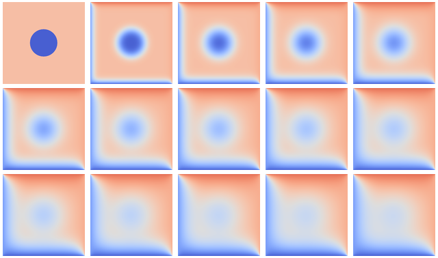
Over time, the temperature distribution progresses from the initial state toward an end state where upper triangle is warm and lower is cold. The average temperature tends to (70 + 85 + 20 + 5) / 4 = 45.

Technique: stencil computation

Heat transfer in the system above is governed by the partial differential equation(s) describing local variation of the temperature field in time and space. That is, the rate of change of the temperature field \(u(x, y, t)\) over two spatial dimensions \(x\) and \(y\) and time \(t\) (with rate coefficient \(\alpha\)) can be modelled via the equation

\[\frac{\partial u}{\partial t} = \alpha \left( \frac{\partial^2 u}{\partial x^2} + \frac{\partial^2 u}{\partial x^2}\right)\]

The standard way to numerically solve differential equations is to discretize them, i. e. to consider only a set/ grid of specific area points at specific moments in time. That way, partial derivatives \({\partial u}\) are converted into differences between adjacent grid points \(u^{m}(i,j)\), with \(m, i, j\) denoting time and spatial grid points, respectively. Temperature change in time at a certain point can now be computed from the values of neighboring points at earlier time; the same expression, called stencil, is applied to every point on the grid.

This simplified model uses an 8x8 grid of data in light blue in state \(m\), each location of which has to be updated based on the indicated 5-point stencil in yellow to move to the next time point \(m+1\).

The following series of exercises uses this stencil example implemented in Julia. The source files listed below represent a simplification of this HeatEquation package, which in turn is inspired by this educational repository containing C/C++/Fortran versions with different parallelization strategies (credits to CSC Finland) (you can also find the source files in the content/code/stencil/ directory of this repository).

main.jlcore.jlheat.jlProject.toml

#using Plots
using BenchmarkTools

include("heat.jl")
include("core.jl")


"""
    visualize(curr::Field, filename=:none)

Create a heatmap of a temperature field. Optionally write png file. 
"""    
function visualize(curr::Field, filename=:none)
    background_color = :white
    plot = heatmap(
        curr.data,
        colorbar_title = "Temperature (C)",
        background_color = background_color
    )

    if filename != :none
        savefig(filename)
    else
        display(plot)
    end
end


ncols, nrows = 2048, 2048
nsteps = 10

# initialize current and previous states to the same state
curr, prev = initialize(ncols, nrows)

# visualize initial field, requires Plots.jl
#visualize(curr, "initial.png")

# simulate temperature evolution for nsteps
simulate!(curr, prev, nsteps)

# visualize final field, requires Plots.jl
#visualize(curr, "final.png")

Run the code

• Copy the source files from the code box above.

• Activate the environment found in the Project.toml file.

• Run the main.jl code and (optionally) visualise the result by uncommenting the relevant line.

• Study the code for a while to understand how it works.

Optimise and benchmark

• Benchmark the evolve!() function in the Julia REPL.

• Add the @inbounds macro to the innermost loop.

• Benchmark again and estimate the performance gain.

Solution

• Add the @btime macro and execute in VSCode:

  @btime simulate!(curr, prev, nsteps)
  

Multithread

• Multithread the evolve!() function

• Benchmark again with different number of threads. It will be most convenient to run these benchmarks from the command line where you can set the number of threads: julia -t <nthreads>.

• How does it scale?

Solution

function evolve!(curr::Field, prev::Field, a, dt)
    Threads.@threads for j = 2:curr.ny+1
        for i = 2:curr.nx+1
            @inbounds xderiv = (prev.data[i-1, j] - 2.0 * prev.data[i, j] + prev.data[i+1, j]) / curr.dx^2
            @inbounds yderiv = (prev.data[i, j-1] - 2.0 * prev.data[i, j] + prev.data[i, j+1]) / curr.dy^2
            @inbounds curr.data[i, j] = prev.data[i, j] + a * dt * (xderiv + yderiv)
        end
    end
end

Running benchmarking from terminal:

$ julia --project -t 1 main.jl
#   1.088 s (4032 allocations: 64.35 MiB)
$ julia --project -t 2 main.jl
#   612.132 ms (7009 allocations: 64.62 MiB)
$ julia --project -t 4 main.jl
#   474.350 ms (13294 allocations: 65.19 MiB)

The scaling isn’t very good because the loops in evolve! are rather cheap.

Adapt the stencil problem for GPU porting

In order to prepare for porting the stencil problem to run on a GPU, it’s wise to modify the code slightly. One approach is to change the evolve! function to accept arrays instead of Field types. For now, we define a new version of this function called evolve2():

function evolve2!(currdata::AbstractArray, prevdata::AbstractArray, dx, dy, a, dt)
    nx, ny = size(currdata) .- 2
    for j = 2:ny+1
        for i = 2:nx+1
            @inbounds xderiv = (prevdata[i-1, j] - 2.0 * prevdata[i, j] + prevdata[i+1, j]) / dx^2
            @inbounds yderiv = (prevdata[i, j-1] - 2.0 * prevdata[i, j] + prevdata[i, j+1]) / dy^2
            @inbounds currdata[i, j] = prevdata[i, j] + a * dt * (xderiv + yderiv)
        end
    end
end

• In the simulate!() function, update how you call the evolve2!() function.

• Take a moment to study the initialize() function. Why is the if arraytype != Matrix statement there?

Solution

In the simulate!() function you need to change from:

evolve!(curr, prev, a, dt)

to:

evolve2!(curr.data, prev.data, curr.dx, curr.dy, a, dt)

The purpose of the if-else block in initialize() is to handle situations where you want the data arrays in the Field composite types to be something else than regular Matrix types. This will be needed when we port to GPU, and also when using SharedArrays.

Using SharedArrays with stencil problem

Look again at the double for-loop in the modified evolve! function and think about how you could use SharedArrays. Start from the evolve2!() function defined above, and try to implement a version that accepts SharedArray arrays.

Hints

• In your main script, import also Distributed and SharedArrays.

• In core.jl, create another method for the evolve2! function with the following signature: evolve2!(currdata::SharedArray, prevdata::SharedArray, dx, dy, a, dt)

• The only change you have to make to the SharedArray method of evolve2!() is to add @sync @distributed in front of the first loop!

Solution and benchmarking

This is how the SharedArray method should look:

function evolve2!(currdata::SharedArray, prevdata::SharedArray, dx, dy, a, dt)
    nx, ny = size(currdata) .- 2
    @sync @distributed for j = 2:ny+1
        for i = 2:nx+1
            @inbounds xderiv = (prevdata[i-1, j] - 2.0 * prevdata[i, j] + prevdata[i+1, j]) / dx^2
            @inbounds yderiv = (prevdata[i, j-1] - 2.0 * prevdata[i, j] + prevdata[i, j+1]) / dy^2
            @inbounds currdata[i, j] = prevdata[i, j] + a * dt * (xderiv + yderiv)
        end
    end
end

and this is how you would set up the simulation in the main file:

using BenchmarkTools
using Distributed
using SharedArrays
include("heat.jl")
include("core.jl")
# ... definition of visualize()
ncols, nrows = 2048, 2048
nsteps = 10
curr, prev = initialize(ncols, nrows, SharedArray)
@btime simulate!(curr, prev, nsteps)

To run the script with multiple processes:

$ julia -p 4 --project main.jl

NOTE: Your benchmark results will turn out to be underwhelming - the SharedArray version will most likely run slower! See explanation below.

Notes on performance

• The overhead in managing the workers will probably far outweigh the parallelisation benefit because the computation in the inner loop is very simple and extremely fast.

• To see the benefit you can obtain for more computationally demanding calculations, you can try to introduce a more expensive mathematical operation to the inner loop, e.g. by taking the arctangent of some values:

  @inbounds xderiv = (atan(prevdata[i-1, j]) - 2.0 * atan(prevdata[i, j]) + atan(prevdata[i+1, j])) / dx^2
  @inbounds yderiv = (atan(prevdata[i, j-1]) - 2.0 * atan(prevdata[i, j]) + atan(prevdata[i, j+1])) / dy^2
  

This should clearly demonstrate the performance benefit of parallelisation via SharedArrays:

$ julia -p 1 --project main.jl
#    1.840 s (442 allocations: 64.03 MiB)
$ julia -p 4 --project main.jl
#    513.529 ms (8315 allocations: 64.39 MiB)

Exercise: Julia port to GPUs

Carefully inspect all Julia source files and consider the following questions:

1. Which functions should be ported to run on GPU?

2. Try to start sketching GPU-ported versions of the key functions.

3. When you have a version running on a GPU (your own or the solution provided below), try benchmarking it by adding @btime in front of simulate!() in main.jl. Benchmark also the CPU version, and compare.

Further considerations:

1. The kernel function needs to end with return or return nothing.

2. The arrays are two-dimensional, so you will need both the .x and .y parts of threadIdx(), blockDim() and blockIdx().

   • Does it matter how you match the x and y dimensions of the threads and blocks to the dimensions of the data (i.e. rows and columns)?

3. You also need to specify tuples for the number of threads and blocks in the x and y dimensions, e.g. threads = (32, 32) and similarly for blocks (using cld).

   • Note the hardware limitations: the product of x and y threads cannot exceed it.

4. For debugging, you can print from inside a kernel using @cuprintln (e.g. to print thread numbers). It will only print during the first execution - redefine the function again to print again. If you get warnings or errors relating to types, you can use the code introspection macro @device_code_warntype to see the types inferred by the compiler.

5. Check correctness of your results! To test that evolve! and evolve_gpu! give (approximately) the same results, for example:

Hints

• create a new function evolve_gpu!() which contains the GPU kernelized version of evolve!()

• in the loop over timesteps in simulate!(), you will need a conditional like if typeof(curr.data) <: ROCArray to call your GPU-ported function

• you cannot pass the struct Field to the kernel. You will instead need to directly pass the array Field.data. This also necessitates passing in other variables like curr.dx^2, etc.

More hints

• since the data is two-dimensional, you’ll need i = (blockIdx().x - 1) * blockDim().x + threadIdx().x and j = (blockIdx().y - 1) * blockDim().y + threadIdx().y

• to not overindex the 2D array, you can use a conditional like if i > 1 && j > 1 && i < nx+2 && j < ny+2

• when calling the kernel, you can set the number of threads and blocks like xthreads = ythreads = 16 and xblocks, yblocks = cld(curr.nx, xthreads), cld(curr.ny, ythreads), and then call it with, e.g., @roc threads=(xthreads, ythreads) blocks = (xblocks, yblocks) evolve_rocm!(curr.data, prev.data, curr.dx^2, curr.dy^2, nx, ny, a, dt).

Solution

1. The evolve!() and simulate!() functions need to be ported. The main.jl file also needs to be updated to work with GPU arrays.

2. “Scalar indexing” is where you iterate over a GPU array, which would be excruciatingly slow and is indeed only allowed in interactive REPL sessions. Without the if-statements in the initialize!() function, the generate_field!() method would be doing disallowed scalar indexing if you were running on a GPU.

3. The GPU-ported version is found below. Try it out on both CPU and GPU and observe the speedup. Play around with array size to see if the speedup is affected. You can also play around with the xthreads and ythreads variables to see if it changes anything.

main_gpu.jlcore_gpu.jl

#using Plots
using BenchmarkTools
using AMDGPU

include("heat.jl")
include("core_gpu.jl")


"""
    visualize(curr::Field, filename=:none)

Create a heatmap of a temperature field. Optionally write png file. 
"""    
function visualize(curr::Field, filename=:none)
    background_color = :white
    plot = heatmap(
        curr.data,
        colorbar_title = "Temperature (C)",
        background_color = background_color
    )

    if filename != :none
        savefig(filename)
    else
        display(plot)
    end
end


ncols, nrows = 2048, 2048
nsteps = 500

# initialize data on CPU
curr, prev = initialize(ncols, nrows, ROCArray)
# initialize data on CPU
#curr, prev = initialize(ncols, nrows)

# visualize initial field, requires Plots.jl
#visualize(curr, "initial.png")

# simulate temperature evolution for nsteps
@btime simulate!(curr, prev, nsteps)

# visualize final field, requires Plots.jl
#visualize(curr, "final.png")

dx = dy = 0.01
a = 0.5
nx = ny = 10000
dt = dx^2 * dy^2 / (2.0 * a * (dx^2 + dy^2))
A1 = rand(nx, ny);
A2 = rand(nx, ny);
A1_d = CuArray(A1)
A2_d = CuArray(A2)

evolve!(A1, A2, dx, dy, a, dt)

evolve_gpu!(A1_d, A2_d, dx, dy, a, dt)

all(A1 .≈ Array(A1_d))

1. Perform some benchmarking of the evolve! and evolve_gpu! functions for arrays of various sizes and with different choices of nthreads. You will need to prefix the kernel execution with the CUDA.@sync macro to let the CPU wait for the GPU kernel to finish (otherwise you would be measuring the time it takes to only launch the kernel):

2. Compare your Julia code with the corresponding CUDA version to enjoy the (relative) simplicity of Julia!

Solution

This is one possible GPU kernel version of evolve!:

function evolve_gpu!(currdata, prevdata, dx2, dy2, a, dt)
    nx, ny = size(currdata) .- 2
    # which index (i or j) you assign to x and y matters enormously!
    i = (blockIdx().x - 1) * blockDim().x + threadIdx().x
    j = (blockIdx().y - 1) * blockDim().y + threadIdx().y
    #@cuprintln("threads $i $j") #only for debugging!
    if i > 1 && j > 1 && i < nx+2 && j < ny+2
        @inbounds xderiv = (prevdata[i-1, j] - 2.0 * prevdata[i, j] + prevdata[i+1, j]) / dx2
        @inbounds yderiv = (prevdata[i, j-1] - 2.0 * prevdata[i, j] + prevdata[i, j+1]) / dy2
        @inbounds currdata[i, j] = prevdata[i, j] + a * dt * (xderiv + yderiv)
    end
    return nothing
end

To test it:

dx = dy = 0.01
a = 0.5
nx = ny = 1000
dt = dx^2 * dy^2 / (2.0 * a * (dx^2 + dy^2))
M1 = rand(nx, ny);
M2 = rand(nx, ny);

# copy to GPU and convert to Float32
M1_d = CuArray(cu(M1))
M2_d = CuArray(cu(M2))

# set number of threads and blocks
nthreads = 16
numblocks = cld(nx, nthreads)

# call cpu and gpu versions
evolve!(M1, M2, dx, dy, a, dt)
@cuda threads=(nthreads, nthreads) blocks=(numblocks, numblocks) evolve_gpu!(M1_d, M2_d, dx^2, dy^2, a, dt)

# element-wise comparison
all(M1 .≈ Array(M1_d))

To benchmark:

using BenchmarkTools
@btime evolve!(M1, M2, dx, dy, a, dt)
@btime CUDA.@sync @cuda threads=(nthreads, nthreads) blocks=(numblocks, numblocks) evolve_gpu!(M1_d, M2_d, dx^2, dy^2, a, dt)

Create a package

Take the code for the stencil example and convert it into a Julia package! Instructions for creating Julia packages are found in the Introduction to Julia lesson.

Also try to write one or more tests. It can include unit tests, integration tests or an end-to-end test.

Solution

See HeatEquation.jl.