Expressing parallelism with SYCL: basic data-parallel kernels
Questions
How do we write parallel kernels in SYCL?
Objectives
Learn the difference between task and data parallelism.
Learn about work-items, work-groups, and ND-ranges.
We should have acquired a good enough understanding of the anatomy of a SYCL
program: queues, kernels, and memory management strategies. We have, however,
not really discussed about strategies for expressing parallelism in a SYCL
program. Indeed, the kernels that we have seen and written so far in the exercises
always used a 1-dimensional work distribution, exemplified by the use of
range<1> and id<1> objects as arguments of parallel_for and the
kernel lambdas, respectively.
Our particular problem domain might have additional structure and our program
might benefit, in terms of performance, from exploiting it.
Data and task parallelism [*]
The are two types of parallelism that can be explored and exploited:
- Data parallelism
The data can be distributed across computational units that can run in parallel. Each unit processes the data applying the same or very similar operations to different data elements. A common example is applying a blur filter to an image: the same function is applied to all the pixels the image is made of. This parallelism is natural for the GPU, where the same instruction set is executed in multiple threads.
- Task parallelism
When an application consists of many tasks that perform different operations with (the same or) different data. An example of task parallelism is cooking: slicing vegetables and grilling are very different tasks and can be done at the same time, if more cooks are available. Note that the tasks can consume totally different resources, for example a CPU and a GPU, adding yet another dimension for performance optimization.
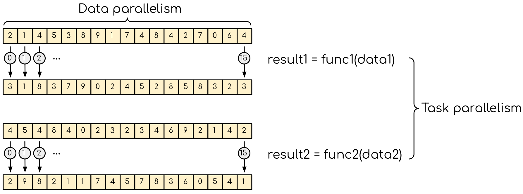
Data parallelism and task parallelism. We have data parallelism when the same operation applies to multiple data, e.g. multiple elements of an array are transformed. Task parallelism implies that there are more than one independent task that, in principle, can be executed in parallel.
In SYCL, we can largely delegate task parallelism to the runtime scheduler:
actions on queues will be arranged in a DAG and tasks that are independent may
execute in an overlapping fashion. Episode The task graph: data, dependencies, synchronization
will show how to gain more direct control.
The parallel_for function is the basic data-parallel construct in SYCL and it accepts two arguments: an execution range and a kernel function.
Based on the way we specify the execution range, we can distinguish three
flavors of data-parallel kernels in SYCL:
basic: when execution is parameterized over a 1-, 2- or 3-dimensional
rangeobject. As the name suggests, simple kernels do not provide control over low-level features, for example, control over the locality of memory accesses.simple
parallel_fortemplate <typename KernelName, int Dims, typename... Rest> event parallel_for(range<Dims> numWorkItems, Rest&&... rest);
ND-range: when execution is parameterized over a 1-, 2-, or 3-dimensional
nd_rangeobject. While superficially similar to simple kernels, the use ofnd_rangewill allow you to group instances of the kernel together. You will gain more flexible control over locality and mapping to hardware resources.ND-range
parallel_fortemplate <typename KernelName, int Dims, typename... Rest> event parallel_for(nd_range<Dims> executionRange, Rest&&... rest);
hierarchical: these form allows to nest kernel invocations, affording some simplifications with respect to ND-range kernels. We will not discuss hierarchical parallel kernels. This is a fast-changing area in the standard: support in various implementation varies and may not work properly.
Note
A data-parallel kernel is not a loop. When we launch a kernel through a
parallel_for, the runtime will instantiate the same operation over all
data elements in the execution range. These instances run in parallel (but
not necessarily in lockstep!) As such, a data-parallel kernel is not
performing any iterations and should be viewed as a descriptive abstraction
on top of the execution model and the backend.
Basic data-parallel kernels
Basic data-parallel kernels are the most suited for embarassing data
parallelism, such as the blurring filter example above. The first argument to
the parallel_for invocation is the execution range, represented by a
range object in 1-, 2-, or 3-dimensions. A range is a grid of work-items of
type item, each item is an instance of the kernel and is uniquely
addressable through objects of id type. \(N\)-dimensional ranges are
arranged in row-major order: dimension \(N-1\) is contiguous.

A range<2> object, representing a 2-dimensional execution range. Each
element in the range is of type item<2> and is indexed by an object of
type id<2>. Items are instances of the kernel. An \(N\)-dimensional
range is in row-major order: dimension \(N-1\) is contiguous.
Figure adapted from [RAB+21].
In basic data-parallel kernels, the kernel function passed as second argument to
the parallel_for invocation can accept either objects of id or of
item type.
In all cases, the range class describes the sizes of both buffers and
execution range of the kernel.
When to use id and when to use item as arguments in the kernel function?
id knows about the individual kernel instance only.
In this kernel, we set all elements in a 2-dimensional array to the magic
value of 42. This is embarrassingly parallel and each instance of the kernel
only needs access to one element in the buffer, indexed by the id of the
instance.
Q.submit([&](handler &cgh) {
  accessor acc { buf, cgh, write_only };

  cgh.parallel_for(range<2> { n_work_items }, [=](id<2> idx) {
    acc[idx] = 42.0;
  });
});
item knows about the individual kernel instance and the global execution range.
In this kernel, we sum two vectors using a 1-dimensional execution range.
Passing item<1> as argument to the kernel lets us probe the global index
of the individual kernel instance in the parallel_for. We use it to index
our accessors to the buffers.
Q.submit([&](handler& cgh) {
  auto accA = bufA.get_access<access::mode::read>(cgh);
  auto accB = bufB.get_access<access::mode::read>(cgh);
  auto accR = bufR.get_access<access::mode::write>(cgh);

  cgh.parallel_for(range { dataSize }, [=](item<1> itm) {
    auto globalId  = itm.get_id();
    accR[globalId] = accA[globalId] + accB[globalId];
  });
});
Naïve MatMul
Let’s now write a data-parallel kernel of the basic flavor to perform a
matrix multiplication. Given the problem, buffer s, accessor s,
range s, and id s will all be 2-dimensional.

Schematics of a naïve implementation of matrix multiplication: \(C_{ij} = \sum_{k}A_{ik}B_{kj}\). Each kernel instance will compute an element in the result matrix \(\mathbf{C}\) by accessing a full row of \(\mathbf{A}\) and a full column of \(\mathbf{B}\). Figure adapted from [RAB+21].
Don’t do this at home, use optimized BLAS!
You can find a scaffold for the code in the
content/code/day-2/00_range-matmul/range-matmul.cpp file,
alongside the CMake script to build the executable. You will have to complete
the source code to compile and run correctly: follow the hints in the source
file. A working solution is in the solution subfolder.
We first create a queue and map it to the GPU, either explicitly:
queue Q{gpu_selector{}};
or implicitly, by compiling with the appropriate
HIPSYCL_TARGETSvalue.We declare the operands as
std::vector<double>the right-hand side operands are filled with random numbers, while the result matrix is zeroed out:std::random_device rd; std::mt19937 mt(rd()); std::uniform_real_distribution<double> dist(0.0, 1.0); std::generate(a.begin(), a.end(), [&dist, &mt]() { return dist(mt); }); std::generate(b.begin(), b.end(), [&dist, &mt]() { return dist(mt); }); std::fill(c.begin(), c.end(), 0.0);
We define buffers to the operands in our matrix multiplication. For example, for the matrix \(\mathbf{A}\):
buffer<double, 2> a_buf(a.data(), range<2>(N, N));
We submit work to the queue through a command group handler:
Q.submit([&](handler& cgh) {
  /* work for the queue */
});
We declare accessors to the buffers. For example, for the matrix \(\mathbf{A}\):
accessor a{ a_buf, cgh };
Within the handler, we launch a
parallel_for. The parallel region iterates over the 2-dimensional range of indices spanned by the output matrix \(\mathbf{C}\) and for every output index pair, performs an iteration over the inner index \(k\):cgh.parallel_for( range{ /* number of rows in C */, /* number of columns in C */ }, [=](id<2> idx){ auto j = idx[0]; auto i = idx[1]; for (auto k = 0; k < N; ++k) { c[j][i] += ...; } } );
Check that your results are correct.
You can find a scaffold for the code in the
content/code/day-2/01_usm-range-matmul/usm-range-matmul.cpp file,
alongside the CMake script to build the executable. You will have to complete
the source code to compile and run correctly: follow the hints in the source
file. A working solution is in the solution subfolder.
We first create a queue and map it to the GPU, either explicitly:
queue Q{gpu_selector{}};
or implicitly, by compiling with the appropriate
HIPSYCL_TARGETSvalue.We allocate the operands as USM buffers and fill them with random numbers. We can do this with untyped or typed
malloc-style orusm_allocatorAPIs. Should operands be host, device, or shared allocations?We allocate the result as USM buffer and zero it out. We can do this with untyped or typed
malloc-style orusm_allocatorAPIs. Should this be host, device, or shared allocation?We submit work to the queue. Note that we need to linearize indices for row-major access to our buffers:
auto irow = ...;
auto jcol = ...;
auto row_major_id = irow * N + jcol;
Check that your results are correct.
Keypoints
The task graph abstraction in SYCL can take care of task parallelism for us.
Data parallelism is achieved with
parallel_forand kernel-based programming.There are three flavors of data-parallel kernels. The basic and ND-range forms are stable in SYCL 2020.
Basic kernels are especially well-suited for embarassing parallelism.
Footnotes