Example: putting it all together
Questions
How do I compile and run code developed using different programming models and frameworks?
What can I expect from the GPU-ported programs in terms of performance gains / trends and how do I estimate this?
Objectives
To show a self-contained example of parallel computation executed on CPU and GPU using different programming models
To show differences and consequences of implementing the same algorithm in natural “style” of different models/ frameworks
To discuss how to assess theoretical and practical performance scaling of GPU codes
Instructor note
35 min teaching
30 min exercises
Problem: heat flow in two-dimensional area
Heat flows in objects according to local temperature differences, as if seeking local equilibrium. The following example defines a rectangular area with two always-warm sides (temperature 70 and 85), two cold sides (temperature 20 and 5) and a cold disk at the center. Because of heat diffusion, temperature of neighboring patches of the area is bound to equalize, changing the overall distribution:
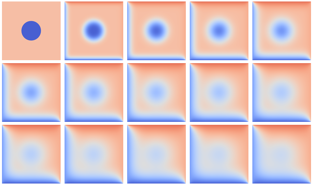
Over time, the temperature distribution progresses from the initial state toward an end state where upper triangle is warm and lower is cold. The average temperature tends to (70 + 85 + 20 + 5) / 4 = 45.
Technique: stencil computation
Heat transfer in the system above is governed by the partial differential equation(s) describing local variation of the temperature field in time and space. That is, the rate of change of the temperature field \(u(x, y, t)\) over two spatial dimensions \(x\) and \(y\) and time \(t\) (with rate coefficient \(\alpha\)) can be modelled via the equation
The standard way to numerically solve differential equations is to discretize them, i. e. to consider only a set/ grid of specific area points at specific moments in time. That way, partial derivatives \({\partial u}\) are converted into differences between adjacent grid points \(u^{m}(i,j)\), with \(m, i, j\) denoting time and spatial grid points, respectively. Temperature change in time at a certain point can now be computed from the values of neighboring points at earlier time; the same expression, called stencil, is applied to every point on the grid.

This simplified model uses an 8x8 grid of data in light blue in state \(m\), each location of which has to be updated based on the indicated 5-point stencil in yellow to move to the next time point \(m+1\).
Question: stencil applications
Stencil computation is a common occurrence in solving numerical problems. Have you already encountered it? Can you think of a problem that could be formulated this way in your field / area of expertise?
Solution
One obvious choice is convolution operation, used in image processing to apply various filter kernels; in some contexts, “convolution” and “stencil” are used almost interchangeably. Other related use is for averaging/ pooling adjacent values.
Technical considerations
1. How fast and/ or accurate can the solution be?
Spatial resolution of the temperature field is controlled by the number/ density of the grid points. As the full grid update is required to proceed from one time point to the next, stencil computation is the main target of parallelization (on CPU or GPU).
Moreover, in many cases the chosen time step cannot be arbitrarily large, otherwise the numerical differentiation will fail, and dense/ accurate grids imply small time steps (see inset below), which makes efficient spatial update even more important.
Optional: stencil expression and time-step limit
Differential equation shown above can be discretized using different schemes. For this example, temperature values at each grid point \(u^{m}(i,j)\) are updated from one time point (\(m\)) to the next (\(m+1\)), using the following expressions:
where
and \(\Delta x\), \(\Delta y\), \(\Delta t\) are step sizes in space and time, respectively.
Time-update schemes often have a limit on the maximum allowed time step \(\Delta t\). For the current scheme, it is equal to
2. What to do with area boundaries?
Naturally, stencil expression can’t be applied directly to the outermost grid points that have no outer neighbors. This can be solved by either changing the expression for those points or by adding an additional layer of grid that is used in computing update, but not updated itself – points of fixed temperature for the sides are being used in this example.
3. How could the algorithm be optimized further?
In an earlier episode, importance of efficient memory access was already stressed. In the following examples, each grid point (and its neighbors) is treated mostly independently; however, this also means that for 5-point stencil each value of the grid point may be read up to 5 times from memory (even if it’s the fast GPU memory). By rearranging the order of mathematical operations, it may be possible to reuse these values in a more efficient way.
Another point to note is that even if the solution is propagated in small time steps, not every step might actually be needed for output. Once some local region of the field is updated, mathematically nothing prevents it from being updated for the second time step – even if the rest of the field is still being recalculated – as long as \(t = m-1\) values for the region boundary are there when needed. (Of course, this is more complicated to implement and would only give benefits in certain cases.)
The following table will aid you in navigating the rest of this section:
Episode guide
Sequential and OpenMP-threaded code in C++, including compilation/ running instructions
Naive GPU parallelization, including SYCL compilation instructions
GPU code with device data management (OpenMP, SYCL)
Python implementation, including running instructions on Google Colab
Julia implementation, including running instructions
Sequential and thread-parallel program in C++
If we assume the grid point values to be truly independent for a single time step, stencil application procedure may be straightforwardly written as a loop over the grid points, as shown below in tab “Stencil update”. (General structure of the program and the default parameter values for the problem model are also provided for reference.) CPU-thread parallelism can then be enabled by a single OpenMP #pragma:
core.cpp
// (c) 2023 ENCCS, CSC and the contributors
#include "heat.h"

// Update the temperature values using five-point stencil
// Arguments:
//   curr: current temperature values
//   prev: temperature values from previous time step
//   a: diffusivity
//   dt: time step
void evolve(field *curr, field *prev, double a, double dt)
{
  // Help the compiler avoid being confused by the structs
  double *currdata = curr->data.data();
  double *prevdata = prev->data.data();
  int nx = prev->nx;
  int ny = prev->ny;

  // Determine the temperature field at next time step
  // As we have fixed boundary conditions, the outermost gridpoints
  // are not updated.
  double dx2 = prev->dx * prev->dx;
  double dy2 = prev->dy * prev->dy;

  // Use OpenMP threads for parallel update of grid values
  #pragma omp parallel for
  for (int i = 1; i < nx + 1; i++) {
    for (int j = 1; j < ny + 1; j++) {
      int ind = i * (ny + 2) + j;
      int ip = (i + 1) * (ny + 2) + j;
      int im = (i - 1) * (ny + 2) + j;
      int jp = i * (ny + 2) + j + 1;
      int jm = i * (ny + 2) + j - 1;
      currdata[ind] = prevdata[ind] + a*dt*
	    ((prevdata[ip] - 2.0*prevdata[ind] + prevdata[im]) / dx2 +
	     (prevdata[jp] - 2.0*prevdata[ind] + prevdata[jm]) / dy2);
    }
  }
}
main.cpp
// Main routine for heat equation solver in 2D.
// (c) 2023 ENCCS, CSC and the contributors
#include <cstdio>
#include <omp.h>
#include "heat.h"
double start_time () { return omp_get_wtime(); }
double stop_time () { return omp_get_wtime(); }
int main(int argc, char **argv)
{
// Set up the solver
int nsteps;
field current, previous;
initialize(argc, argv, ¤t, &previous, &nsteps);
// Output the initial field and its temperature
field_write(¤t, 0);
double average_temp = field_average(¤t);
printf("Average temperature, start: %f\n", average_temp);
// Set diffusivity constant
double a = 0.5;
// Compute the largest stable time step
double dx2 = current.dx * current.dx;
double dy2 = current.dy * current.dy;
double dt = dx2 * dy2 / (2.0 * a * (dx2 + dy2));
// Set output interval
int output_interval = 1500;
// Start timer
double start_clock = start_time();
// Time evolution
for (int iter = 1; iter <= nsteps; iter++) {
evolve(¤t, &previous, a, dt);
if (iter % output_interval == 0) {
field_write(¤t, iter);
}
// Swap current and previous fields for next iteration step
field_swap(¤t, &previous);
}
// Stop timer
double stop_clock = stop_time();
// Output the final field and its temperature
average_temp = field_average(&previous);
printf("Average temperature at end: %f\n", average_temp);
// Compare temperature for reference
if (argc == 1) {
printf("Control temperature at end: 59.281239\n");
}
field_write(&previous, nsteps);
// Determine the computation time used for all the iterations
printf("Iterations took %.3f seconds.\n", (stop_clock - start_clock));
return 0;
}
heat.h
// Datatype for temperature field
struct field {
    // nx and ny are the dimensions of the field. The array data
    // contains also ghost layers, so it will have dimensions nx+2 x ny+2
    int nx;
    int ny;
    // Size of the grid cells
    double dx;
    double dy;
    // The temperature values in the 2D grid
    std::vector<double> data;
};

// CONSTANTS
// Fixed grid spacing
const double DX = 0.01;
const double DY = 0.01;
// Default temperatures
const double T_DISC = 5.0;
const double T_AREA = 65.0;
const double T_UPPER = 85.0;
const double T_LOWER = 5.0;
const double T_LEFT = 20.0;
const double T_RIGHT = 70.0;
// Default problem size
const int ROWS = 2000;
const int COLS = 2000;
const int NSTEPS = 500;
Optional: compiling the executables
To compile executable files for the OpenMP-based variants, follow the instructions below:
salloc -A project_465002387 -p small-g -N 1 -c 8 -n 1 --gpus-per-node=1 -t 1:00:00

module load LUMI/24.03
module load partition/G
module load rocm/6.0.3
module load PrgEnv-cray/8.5.0

cd base/
make all
Afterwards login into a compute node and test the executables (or just srun <executable> directly):
$ srun --pty bash

$ ./stencil
$ ./stencil_off
$ ./stencil_data

$ exit
If everything works well, the output should look similar to this:
$ ./stencil
Average temperature, start: 59.763305
Average temperature at end: 59.281239
Control temperature at end: 59.281239
Iterations took 0.566 seconds.
$ ./stencil_off
Average temperature, start: 59.763305
Average temperature at end: 59.281239
Control temperature at end: 59.281239
Iterations took 3.792 seconds.
$ ./stencil_data
Average temperature, start: 59.763305
Average temperature at end: 59.281239
Control temperature at end: 59.281239
Iterations took 1.211 seconds.
$
CPU parallelization: timings
(NOTE: for thread-parallel runs it is necessary to request multiple CPU cores. In LUMI-G partitions, this can be done by asking for multiple GPUs; an alternative is to use -C partitions.)
For later comparison, some benchmarks of the OpenMP thread-parallel implementation are provided below:
Job size |
1 CPU core |
32 CPU cores |
|---|---|---|
S:2000 T:500 |
1.402 |
0.064 |
S:2000 T:5000 |
13.895 |
0.538 |
S:2000 T:10000 |
27.753 |
1.071 |
S:4000 T:500 |
5.727 |
0.633 |
S:8000 T:500 |
24.130 |
16.616 |
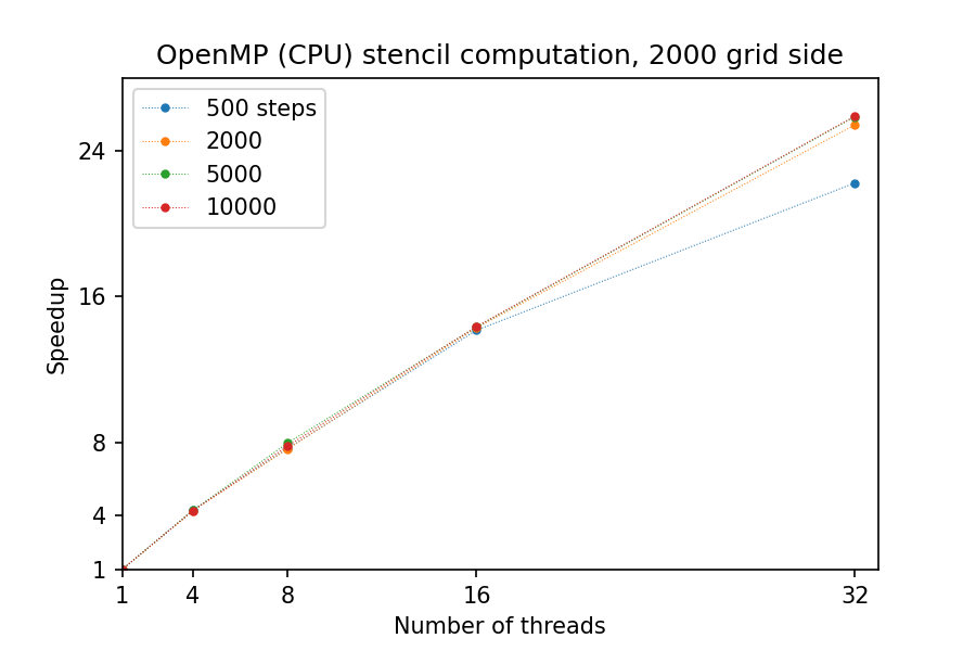
A closer look reveals that the computation time scales very nicely with increasing time steps:
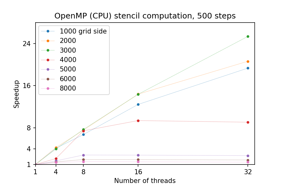
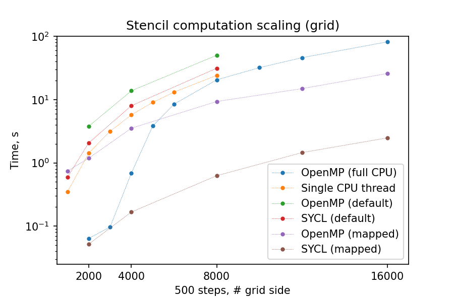
However, for larger grid sizes the parallelization becomes inefficient – as the individual chunks of the grid get too large to fit into CPU cache, threads become bound by the speed of RAM reads/writes:
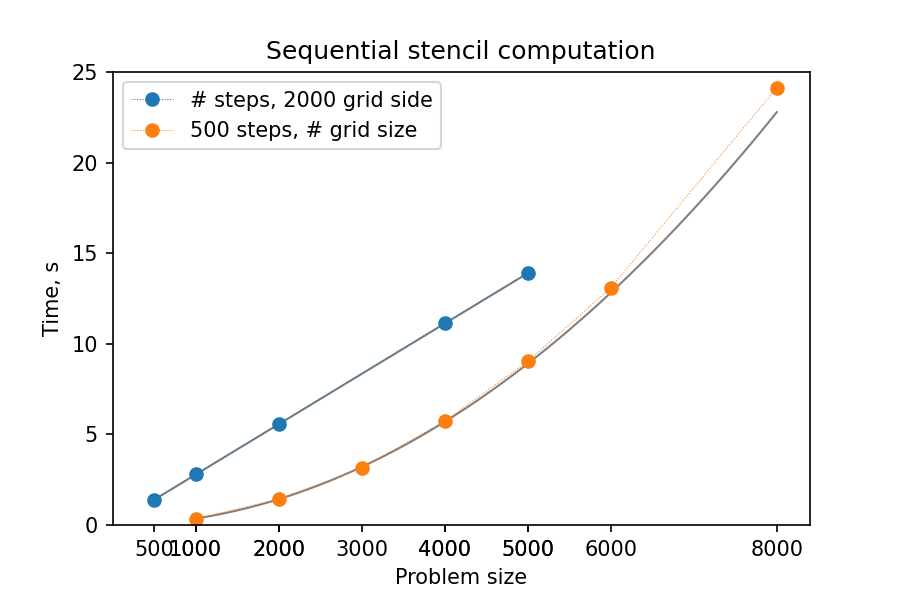
Discussion: heat flow computation scaling
How is heat flow computation expected to scale with respect to the number of time steps?
Linearly
Quadratically
Exponentially
How is stencil application (grid update) expected to scale with respect to the size of the grid side?
Linearly
Quadratically
Exponentially
(Optional) Do you expect GPU-accelerated computations to follow the above-mentioned trends? Why/ why not?
Solution
The answer is a: since each time-step follows the previous one and involves a similar number of operations, then the update time per step will be more or less constant.
The answer is b: since stencil application is independent for every grid point, the update time will be proportional to the number of points, i.e. side * side.
GPU parallelization: first steps
Let’s apply several techniques presented in previous episodes to make stencil update run on GPU.
OpenMP (or OpenACC) offloading requires to define a region to be executed in parallel as well as data that shall be copied over/ used in GPU memory. Similarly, SYCL programming model offers convenient ways to define execution kernels, as well as context to run them in (called queue).
Changes of stencil update code for OpenMP and SYCL are shown in the tabs below:
base/core-off.cpp
// (c) 2023 ENCCS, CSC and the contributors
#include "heat.h"

// Update the temperature values using five-point stencil
// Arguments:
//   curr: current temperature values
//   prev: temperature values from previous time step
//   a: diffusivity
//   dt: time step
void evolve(field *curr, field *prev, double a, double dt)
{
  // Help the compiler avoid being confused by the structs
  double *currdata = curr->data.data();
  double *prevdata = prev->data.data();
  int nx = prev->nx;
  int ny = prev->ny;

  // Determine the temperature field at next time step
  // As we have fixed boundary conditions, the outermost gridpoints
  // are not updated.
  double dx2 = prev->dx * prev->dx;
  double dy2 = prev->dy * prev->dy;

  // Offload value update to GPU target (fallback to CPU is possible)
  #pragma omp target teams distribute parallel for \
  map(currdata[0:(nx+2)*(ny+2)],prevdata[0:(nx+2)*(ny+2)])
  for (int i = 1; i < nx + 1; i++) {
    for (int j = 1; j < ny + 1; j++) {
      int ind = i * (ny + 2) + j;
      int ip = (i + 1) * (ny + 2) + j;
      int im = (i - 1) * (ny + 2) + j;
      int jp = i * (ny + 2) + j + 1;
      int jm = i * (ny + 2) + j - 1;
      currdata[ind] = prevdata[ind] + a*dt*
	    ((prevdata[ip] - 2.0*prevdata[ind] + prevdata[im]) / dx2 +
	     (prevdata[jp] - 2.0*prevdata[ind] + prevdata[jm]) / dy2);
    }
  }
}
sycl/core-naive.cpp
// (c) 2023 ENCCS, CSC and the contributors
#include "heat.h"
#include <sycl/sycl.hpp>

// Update the temperature values using five-point stencil
// Arguments:
//   queue: SYCL queue
//   curr: current temperature values
//   prev: temperature values from previous time step
//   a: diffusivity
//   dt: time step
void evolve(sycl::queue &Q, field *curr, field *prev, double a, double dt) {
  // Help the compiler avoid being confused by the structs
  int nx = prev->nx;
  int ny = prev->ny;
  int size = (nx + 2) * (ny + 2);

  // Determine the temperature field at next time step
  // As we have fixed boundary conditions, the outermost gridpoints
  // are not updated.
  double dx2 = prev->dx * prev->dx;
  double dy2 = prev->dy * prev->dy;

  double *currdata = sycl::malloc_device<double>(size, Q);
  double *prevdata = sycl::malloc_device<double>(size, Q);
  Q.copy<double>(curr->data.data(), currdata, size);
  Q.copy<double>(prev->data.data(), prevdata, size);

  Q.parallel_for(sycl::range<2>(nx, ny), [=](sycl::id<2> id) {
    auto i = id[0] + 1;
    auto j = id[1] + 1;

    int ind = i * (ny + 2) + j;
    int ip = (i + 1) * (ny + 2) + j;
    int im = (i - 1) * (ny + 2) + j;
    int jp = i * (ny + 2) + j + 1;
    int jm = i * (ny + 2) + j - 1;
    currdata[ind] = prevdata[ind] + a*dt*
      ((prevdata[ip] - 2.0*prevdata[ind] + prevdata[im]) / dx2 +
       (prevdata[jp] - 2.0*prevdata[ind] + prevdata[jm]) / dy2);
  });

  Q.copy<double>(currdata, curr->data.data(), size).wait();
  sycl::free(currdata, Q);
  sycl::free(prevdata, Q);
}
Loading SYCL modules on LUMI
As SYCL is placed on top of ROCm/HIP (or CUDA) software stack, running SYCL executables may require respective modules to be loaded. On current nodes, it can be done as follows:
# salloc -A project_465002387 -p small-g -N 1 -c 8 -n 1 --gpus-per-node=1 -t 1:00:00

module load LUMI/24.03
module load partition/G
module load rocm/6.0.3
module use  /appl/local/csc/modulefiles
module load acpp/24.06.0
Optional: compiling the SYCL executables
As previously, you are welcome to generate your own executables:
$ cd ../sycl/
(give the following lines some time, probably a couple of min)
$ acpp -O2 -o stencil_naive core-naive.cpp io.cpp main-naive.cpp pngwriter.c setup.cpp utilities.cpp
$ acpp -O2 -o stencil_data core.cpp io.cpp main.cpp pngwriter.c setup.cpp utilities.cpp

$ srun stencil_naive
$ srun stencil_data
If everything works well, the output should look similar to this:
$ srun stencil_naive
Average temperature, start: 59.763305
Average temperature at end: 59.281239
Control temperature at end: 59.281239
Iterations took 2.086 seconds.
$ srun stencil_data
Average temperature, start: 59.763305
Average temperature at end: 59.281239
Control temperature at end: 59.281239
Iterations took 0.052 seconds.
Exercise: naive GPU ports
Test your compiled executables base/stencil, base/stencil_off and sycl/stencil_naive. Try changing problem size parameters:
srun stencil_naive 2000 2000 5000
Things to look for:
How computation times change?
Do the results align to your expectations?
Solution
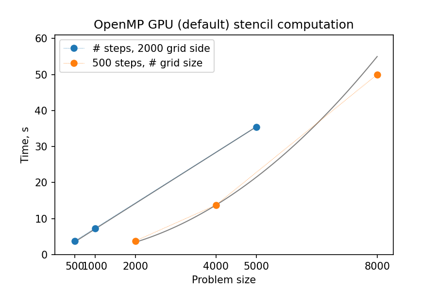
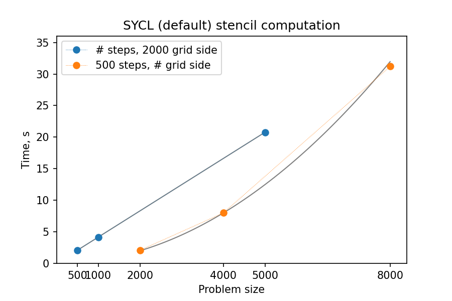
You might notice that the GPU-“ported” versions actually run slower than the single-CPU-core version! In fact, the scaling behavior of all three variants is similar and expected, which is a good sign; only the “computation unit cost” is different. You can compare benchmark summaries in the tabs below:
GPU parallelization: data movement
Why the porting approach above seems to be quite inefficient?
On each step, we:
re-allocate GPU memory,
copy the data from CPU to GPU,
perform the computation,
then copy the data back.
But overhead can be reduced by taking care to minimize data transfers between host and device memory:
allocate GPU memory once at the start of the program,
only copy the data from GPU to CPU when we need it,
swap the GPU buffers between timesteps, like we do with CPU buffers. (OpenMP does this automatically.)
Changes of stencil update code are shown in tabs below (also check out the respective main() functions for calls to persistent GPU buffer creation, access, and deletion):
base/core-data.cpp
// (c) 2023 ENCCS, CSC and the contributors
#include "heat.h"

// Update the temperature values using five-point stencil
// Arguments:
//   curr: current temperature values
//   prev: temperature values from previous time step
//   a: diffusivity
//   dt: time step
void evolve(field *curr, field *prev, double a, double dt)
{
  // Help the compiler avoid being confused by the structs
  double *currdata = curr->data.data();
  double *prevdata = prev->data.data();
  int nx = prev->nx;
  int ny = prev->ny;

  // Determine the temperature field at next time step
  // As we have fixed boundary conditions, the outermost gridpoints
  // are not updated.
  double dx2 = prev->dx * prev->dx;
  double dy2 = prev->dy * prev->dy;

  // Offload value update to GPU target (fallback to CPU is possible)
  #pragma omp target teams distribute parallel for
  for (int i = 1; i < nx + 1; i++) {
    for (int j = 1; j < ny + 1; j++) {
      int ind = i * (ny + 2) + j;
      int ip = (i + 1) * (ny + 2) + j;
      int im = (i - 1) * (ny + 2) + j;
      int jp = i * (ny + 2) + j + 1;
      int jm = i * (ny + 2) + j - 1;
      currdata[ind] = prevdata[ind] + a*dt*
	    ((prevdata[ip] - 2.0*prevdata[ind] + prevdata[im]) / dx2 +
	     (prevdata[jp] - 2.0*prevdata[ind] + prevdata[jm]) / dy2);
    }
  }
}

// Start a data region and copy temperature fields to the device
void enter_data(field *curr, field *prev)
{
  double *currdata = curr->data.data();
  double *prevdata = prev->data.data();
  int nx = prev->nx;
  int ny = prev->ny;

  // adding data mapping here
  #pragma omp target enter data \
  map(to: currdata[0:(nx+2)*(ny+2)], prevdata[0:(nx+2)*(ny+2)])
}

// End a data region and copy temperature fields back to the host
void exit_data(field *curr, field *prev)
{
  double *currdata = curr->data.data();
  double *prevdata = prev->data.data();
  int nx = prev->nx;
  int ny = prev->ny;

  // adding data mapping here
  #pragma omp target exit data \
  map(from: currdata[0:(nx+2)*(ny+2)], prevdata[0:(nx+2)*(ny+2)])
}

// Copy a temperature field from the device to the host
void update_host(field *heat)
{
  double *data = heat->data.data();
  int nx = heat->nx;
  int ny = heat->ny;

  // adding data mapping here
  #pragma omp target update from(data[0:(nx+2)*(ny+2)])
}
sycl/core.cpp
// (c) 2023 ENCCS, CSC and the contributors
#include "heat.h"
#include <sycl/sycl.hpp>

// Update the temperature values using five-point stencil
// Arguments:
//   queue: SYCL queue
//   currdata: current temperature values (device pointer)
//   prevdata: temperature values from previous time step (device pointer)
//   prev: description of the grid parameters
//   a: diffusivity
//   dt: time step
void evolve(sycl::queue &Q, double* currdata, const double* prevdata,
            const field *prev, double a, double dt)
{
  int nx = prev->nx;
  int ny = prev->ny;

  // Determine the temperature field at next time step
  // As we have fixed boundary conditions, the outermost gridpoints
  // are not updated.
  double dx2 = prev->dx * prev->dx;
  double dy2 = prev->dy * prev->dy;

  Q.parallel_for(sycl::range<2>(nx, ny), [=](sycl::id<2> id) {
    auto i = id[0] + 1;
    auto j = id[1] + 1;

    int ind = i * (ny + 2) + j;
    int ip = (i + 1) * (ny + 2) + j;
    int im = (i - 1) * (ny + 2) + j;
    int jp = i * (ny + 2) + j + 1;
    int jm = i * (ny + 2) + j - 1;
    currdata[ind] = prevdata[ind] + a*dt*
      ((prevdata[ip] - 2.0*prevdata[ind] + prevdata[im]) / dx2 +
       (prevdata[jp] - 2.0*prevdata[ind] + prevdata[jm]) / dy2);
  });
}

void copy_to_buffer(sycl::queue Q, double* buffer, const field* f)
{
    int size = (f->nx + 2) * (f->ny + 2);
    Q.copy<double>(f->data.data(), buffer, size);
}

void copy_from_buffer(sycl::queue Q, const double* buffer, field *f)
{
    int size = (f->nx + 2) * (f->ny + 2);
    Q.copy<double>(buffer, f->data.data(), size).wait();
}
Exercise: updated GPU ports
Test your compiled executables base/stencil_data and sycl/stencil_data. Try changing problem size parameters:
srun stencil 2000 2000 5000
Things to look for:
How computation times change this time around?
What largest grid and/or longest propagation time can you get in 10 s on your machine?
Solution
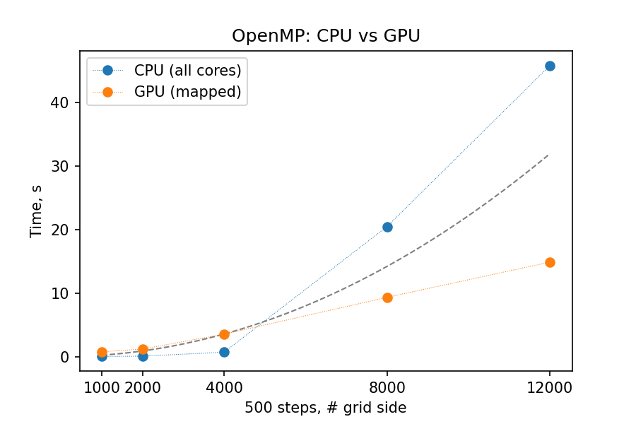
Using GPU offloading with mapped device data, it is possible to achieve performance gains compared to thread-parallel version for larger grid sizes, due to the fact that the latter version becomes essentially RAM-bound, but the former does not.
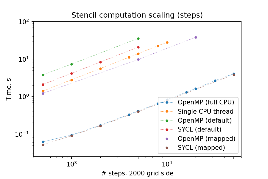
Below you can find the summary graphs for step- and grid- scaling of the stencil update task. Because of the more explicit programming approach, SYCL GPU port is much faster than OpenMP-offloaded version, comparable with thread-parallel CPU version running on all cores of a single node.
Python: JIT and GPU acceleration
As mentioned previously, Numba package allows developers to just-in-time (JIT) compile Python code to run fast on CPUs, but can also be used for JIT compiling for (NVIDIA) GPUs. JIT seems to work well on loop-based, computationally heavy functions, so trying it out is a nice choice for initial source version:
core.py
from numba import jit


# Update the temperature values using five-point stencil
# Arguments:
#   curr: current temperature field object
#   prev: temperature field from previous time step
#   a: diffusivity
#   dt: time step
def evolve(current, previous, a, dt):
    dx2, dy2 = previous.dx**2, previous.dy**2
    curr, prev = current.data, previous.data
    # Run (possibly accelerated) update
    _evolve(curr, prev, a, dt, dx2, dy2)


@jit(nopython=True)
def _evolve(curr, prev, a, dt, dx2, dy2):
    nx, ny = prev.shape # These are the FULL dims, rows+2 / cols+2
    for i in range(1, nx-1):
        for j in range(1, ny-1):
            curr[i, j] = prev[i, j] + a * dt * ( \
              (prev[i+1, j] - 2*prev[i, j] + prev[i-1, j]) / dx2 + \
              (prev[i, j+1] - 2*prev[i, j] + prev[i, j-1]) / dy2 )
heat.py
@jit(nopython=True)
def _generate(data, nx, ny):
    # Radius of the source disc
    radius = nx / 6.0
    for i in range(nx+2):
        for j in range(ny+2):
            # Distance of point i, j from the origin
            dx = i - nx / 2 + 1
            dy = j - ny / 2 + 1
            if (dx * dx + dy * dy < radius * radius):
                data[i,j] = T_DISC
            else:
                data[i,j] = T_AREA

    # Boundary conditions
    for i in range(nx+2):
        data[i,0] = T_LEFT
        data[i, ny+1] = T_RIGHT

    for j in range(ny+2):
        data[0,j] = T_UPPER
        data[nx+1, j] = T_LOWER
core_cuda.py
import math
from numba import cuda

# Update the temperature values using five-point stencil
# Arguments:
#   curr: current temperature field object
#   prev: temperature field from previous time step
#   a: diffusivity
#   dt: time step
def evolve(current, previous, a, dt):
    dx2, dy2 = previous.dx**2, previous.dy**2
    curr, prev = current.dev, previous.dev
    # Set thread and block sizes
    nx, ny = prev.shape # These are the FULL dims, rows+2 / cols+2
    tx, ty = (16, 16)   # Arbitrary choice
    bx, by = math.ceil(nx / tx), math.ceil(ny / ty)
    # Run numba (CUDA) kernel
    _evolve_kernel[(bx, by), (tx, ty)](curr, prev, a, dt, dx2, dy2)


@cuda.jit()
def _evolve_kernel(curr, prev, a, dt, dx2, dy2):
    nx, ny = prev.shape # These are the FULL dims, rows+2 / cols+2
    i, j = cuda.grid(2)
    if ((i >= 1) and (i < nx-1)
        and (j >= 1) and (j < ny-1)):
        curr[i, j] = prev[i, j] + a * dt * ( \
            (prev[i+1, j] - 2*prev[i, j] + prev[i-1, j]) / dx2 + \
            (prev[i, j+1] - 2*prev[i, j] + prev[i, j-1]) / dy2 )
The alternative approach would be to rewrite stencil update code in NumPy style, exploiting loop vectorization.
Short summary of a typical Colab run is provided below:
Job size |
JIT (LUMI) |
JIT (Colab) |
Job size |
no JIT (Colab) |
|---|---|---|---|---|
S:2000 T:500 |
1.648 |
8.495 |
S:200 T:50 |
5.318 |
S:2000 T:200 |
0.787 |
3.524 |
S:200 T:20 |
1.859 |
S:1000 T:500 |
0.547 |
2.230 |
S:100 T:50 |
1.156 |
Numba’s @vectorize and @guvectorize decorators offer an interface to create CPU- (or GPU-) accelerated Python functions without explicit implementation details. However, such functions become increasingly complicated to write (and optimize by the compiler) with increasing complexity of the computations within.
Numba also offers direct CUDA-based kernel programming, which can be the best choice for those already familiar with CUDA. Example for stencil update written in Numba CUDA is shown in the above section, tab “Stencil update in GPU”. In this case, data transfer functions devdata = cuda.to_device(data) and devdata.copy_to_host(data) (see main_cuda.py) are already provided by Numba package.
Exercise: CUDA acceleration in Python
Using Google Colab (or your own machine), run provided Numba-CUDA Python program. Try changing problem size parameters:
args.rows, args.cols, args.nsteps = 2000, 2000, 5000for notebooks,[
srun]python3 main.py 2000 2000 5000for command line.
Things to look for:
How computation times change?
Do you get better performance than from JIT-compiled CPU version? How far can you push the problem size?
Are you able to monitor the GPU usage?
Solution
Some numbers from Colab:
Job size |
JIT (LUMI) |
JIT (Colab) |
CUDA (Colab) |
|---|---|---|---|
S:2000 T:500 |
1.648 |
8.495 |
1.079 |
S:2000 T:2000 |
6.133 |
36.61 |
3.931 |
S:5000 T:500 |
9.478 |
57.19 |
6.448 |
Julia GPU acceleration
A Julia version of the stencil example above can be found below (a simplified version of the HeatEquation module at https://github.com/ENCCS/HeatEquation.jl). The source files are also available in the content/examples/stencil/julia directory of this repository.
To run the example on LUMI CPU partition, type:
$ # interactive CPU node
$ srun --account=project_465002387 --partition=standard --nodes=1 --cpus-per-task=32 --ntasks-per-node=1 --time=01:00:00 --pty bash
$ # load Julia env
$ module purge
$ module use /appl/local/csc/modulefiles
$ module load julia
$ module load julia-amdgpu
$ # in directory with Project.toml and source files, instantiate an environment to install packages
$ julia --project -e "using Pkg ; Pkg.instantiate()"
$ # finally run
$ julia --project main.jl
To run on the GPU partition, use instead the srun command
$ srun --account=project_465002387 --partition=standard-g --nodes=1 --cpus-per-task=1 --ntasks-per-node=1 --gpus-per-node=1 --time=1:00:00 --pty bash
Optional dependency
Note that the Plots.jl dependency is commented out in main.jl and Project.toml. This saves ~2 minute precompilation time when you first instantiate the Julia environment. To generate plots, just uncomment the commented Plots.jl dependency in Project.toml, instantiate again, and import and use Plots in main.jl.
#using Plots
using BenchmarkTools

include("heat.jl")
include("core.jl")


"""
    visualize(curr::Field, filename=:none)

Create a heatmap of a temperature field. Optionally write png file.
"""
function visualize(curr::Field, filename=:none)
    background_color = :white
    plot = heatmap(
        curr.data,
        colorbar_title = "Temperature (C)",
        background_color = background_color
    )

    if filename != :none
        savefig(filename)
    else
        display(plot)
    end
end


ncols, nrows = 2048, 2048
nsteps = 500

# initialize current and previous states to the same state
curr, prev = initialize(ncols, nrows)

# visualize initial field, requires Plots.jl
#visualize(curr, "initial.png")

# simulate temperature evolution for nsteps
simulate!(curr, prev, nsteps)

# visualize final field, requires Plots.jl
#visualize(curr, "final.png")
using ProgressMeter

"""
    evolve!(curr::Field, prev::Field, a, dt)

Calculate a new temperature field curr based on the previous
field prev. a is the diffusion constant and dt is the largest
stable time step.
"""
function evolve!(curr::Field, prev::Field, a, dt)
    Threads.@threads for j = 2:curr.ny+1
        for i = 2:curr.nx+1
            @inbounds xderiv = (prev.data[i-1, j] - 2.0 * prev.data[i, j] + prev.data[i+1, j]) / curr.dx^2
            @inbounds yderiv = (prev.data[i, j-1] - 2.0 * prev.data[i, j] + prev.data[i, j+1]) / curr.dy^2
            @inbounds curr.data[i, j] = prev.data[i, j] + a * dt * (xderiv + yderiv)
        end
    end
end


"""
    swap_fields!(curr::Field, prev::Field)

Swap the data of two fields curr and prev.
"""
function swap_fields!(curr::Field, prev::Field)
    tmp = curr.data
    curr.data = prev.data
    prev.data = tmp
end

"""
    average_temperature(f::Field)

Calculate average temperature of a temperature field.
"""
average_temperature(f::Field) = sum(f.data[2:f.nx+1, 2:f.ny+1]) / (f.nx * f.ny)

"""
    simulate!(current, previous, nsteps)

Run the heat equation solver on fields curr and prev for nsteps.
"""
function simulate!(curr::Field, prev::Field, nsteps)

    println("Initial average temperature: $(average_temperature(curr))")

    # Diffusion constant
    a = 0.5
    # Largest stable time step
    dt = curr.dx^2 * curr.dy^2 / (2.0 * a * (curr.dx^2 + curr.dy^2))

    # display a nice progress bar
    p = Progress(nsteps)

    for i = 1:nsteps
        # calculate new state based on previous state
        evolve!(curr, prev, a, dt)

        # swap current and previous fields
        swap_fields!(curr, prev)

        # increment the progress bar
        next!(p)
    end

    # print final average temperature
    println("Final average temperature: $(average_temperature(curr))")
end
# Fixed grid spacing
const DX = 0.01
const DY = 0.01
# Default temperatures
const T_DISC = 5.0
const T_AREA = 65.0
const T_UPPER = 85.0
const T_LOWER = 5.0
const T_LEFT = 20.0
const T_RIGHT = 70.0
# Default problem size
const ROWS = 2000
const COLS = 2000
const NSTEPS = 500


"""
    Field(nx::Int64, ny::Int64, dx::Float64, dy::Float64, data::Matrix{Float64})

Temperature field type. nx and ny are the dimensions of the field.
The array data contains also ghost layers, so it will have dimensions
[nx+2, ny+2]
"""
mutable struct Field{T<:AbstractArray}
    nx::Int64
    ny::Int64
    # Size of the grid cells
    dx::Float64
    dy::Float64
    # The temperature values in the 2D grid
    data::T
end

# outer constructor with default cell sizes and initialized data
Field(nx::Int64, ny::Int64, data) = Field{typeof(data)}(nx, ny, 0.01, 0.01, data)

# extend deepcopy to new type
Base.deepcopy(f::Field) = Field(f.nx, f.ny, f.dx, f.dy, deepcopy(f.data))

"""
    initialize(rows::Int, cols::Int, arraytype = Matrix)

Initialize two temperature field with (nrows, ncols) number of
rows and columns. If the arraytype is something else than Matrix,
create data on the CPU first to avoid scalar indexing errors.
"""
function initialize(nrows = 1000, ncols = 1000, arraytype = Matrix)
    data = zeros(nrows+2, ncols+2)

    # generate a field with boundary conditions
    if arraytype != Matrix
        tmp = Field(nrows, ncols, data)
        generate_field!(tmp)
        gpudata = arraytype(tmp.data)
        previous = Field(nrows, ncols, gpudata)
    else
        previous = Field(nrows, ncols, data)
        generate_field!(previous)
    end

    current = Base.deepcopy(previous)

    return previous, current
end


"""
    generate_field!(field0::Field)

Generate a temperature field.  Pattern is disc with a radius
of nx / 6 in the center of the grid. Boundary conditions are
(different) constant temperatures outside the grid.
"""
function generate_field!(field::Field)
    # Square of the disk radius
    radius2 = (field.nx / 6.0)^2

    for j = 1:field.ny+2
        for i = 1:field.nx+2
            ds2 = (i - field.nx / 2)^2 + (j - field.ny / 2)^2
            if ds2 < radius2
                field.data[i,j] = T_DISC
            else
                field.data[i,j] = T_AREA
            end
        end
    end

    # Boundary conditions
    field.data[:,1] .= T_LEFT
    field.data[:,field.ny+2] .= T_RIGHT
    field.data[1,:] .= T_UPPER
    field.data[field.nx+2,:] .= T_LOWER
end
[deps]
BenchmarkTools = "6e4b80f9-dd63-53aa-95a3-0cdb28fa8baf"
#Plots = "91a5bcdd-55d7-5caf-9e0b-520d859cae80"
ProgressMeter = "92933f4c-e287-5a05-a399-4b506db050ca"
Exercise: Julia port to GPUs
Carefully inspect all Julia source files and consider the following questions:
Which functions should be ported to run on GPU?
Look at the
initialize!()function and how it uses thearraytypeargument. This could be done more compactly and elegantly, but this solution solves scalar indexing errors. What are scalar indexing errors?Try to start sketching GPU-ported versions of the key functions.
When you have a version running on a GPU (your own or the solution provided below), try benchmarking it by adding
@btimein front ofsimulate!()inmain.jl. Benchmark also the CPU version, and compare.
Hints
create a new function
evolve_gpu!()which contains the GPU kernelized version ofevolve!()in the loop over timesteps in
simulate!(), you will need a conditional likeif typeof(curr.data) <: ROCArrayto call your GPU-ported functionyou cannot pass the struct
Fieldto the kernel. You will instead need to directly pass the arrayField.data. This also necessitates passing in other variables likecurr.dx^2, etc.
More hints
since the data is two-dimensional, you’ll need
i = (blockIdx().x - 1) * blockDim().x + threadIdx().xandj = (blockIdx().y - 1) * blockDim().y + threadIdx().yto not overindex the 2D array, you can use a conditional like
if i > 1 && j > 1 && i < nx+2 && j < ny+2when calling the kernel, you can set the number of threads and blocks like
xthreads = ythreads = 16andxblocks, yblocks = cld(curr.nx, xthreads), cld(curr.ny, ythreads), and then call it with, e.g.,@roc threads=(xthreads, ythreads) blocks = (xblocks, yblocks) evolve_rocm!(curr.data, prev.data, curr.dx^2, curr.dy^2, nx, ny, a, dt).
Solution
The
evolve!()andsimulate!()functions need to be ported. Themain.jlfile also needs to be updated to work with GPU arrays.“Scalar indexing” is where you iterate over a GPU array, which would be excruciatingly slow and is indeed only allowed in interactive REPL sessions. Without the if-statements in the
initialize!()function, thegenerate_field!()method would be doing disallowed scalar indexing if you were running on a GPU.The GPU-ported version is found below. Try it out on both CPU and GPU and observe the speedup. Play around with array size to see if the speedup is affected. You can also play around with the
xthreadsandythreadsvariables to see if it changes anything.
#using Plots
using BenchmarkTools
using AMDGPU

include("heat.jl")
include("core_gpu.jl")


"""
    visualize(curr::Field, filename=:none)

Create a heatmap of a temperature field. Optionally write png file.
"""
function visualize(curr::Field, filename=:none)
    background_color = :white
    plot = heatmap(
        curr.data,
        colorbar_title = "Temperature (C)",
        background_color = background_color
    )

    if filename != :none
        savefig(filename)
    else
        display(plot)
    end
end


ncols, nrows = 2048, 2048
nsteps = 500

# initialize data on CPU
curr, prev = initialize(ncols, nrows, ROCArray)
# initialize data on CPU
#curr, prev = initialize(ncols, nrows)

# visualize initial field, requires Plots.jl
#visualize(curr, "initial.png")

# simulate temperature evolution for nsteps
@btime simulate!(curr, prev, nsteps)

# visualize final field, requires Plots.jl
#visualize(curr, "final.png")
using ProgressMeter

"""
    evolve!(curr::Field, prev::Field, a, dt)

Calculate a new temperature field curr based on the previous
field prev. a is the diffusion constant and dt is the largest
stable time step.
"""
function evolve!(curr::Field, prev::Field, a, dt)
    Threads.@threads for j = 2:curr.ny+1
        for i = 2:curr.nx+1
            @inbounds xderiv = (prev.data[i-1, j] - 2.0 * prev.data[i, j] + prev.data[i+1, j]) / curr.dx^2
            @inbounds yderiv = (prev.data[i, j-1] - 2.0 * prev.data[i, j] + prev.data[i, j+1]) / curr.dy^2
            @inbounds curr.data[i, j] = prev.data[i, j] + a * dt * (xderiv + yderiv)
        end
    end
end


function evolve_cuda!(currdata, prevdata, dx2, dy2, nx, ny, a, dt)
    i = (blockIdx().x - 1) * blockDim().x + threadIdx().x
    j = (blockIdx().y - 1) * blockDim().y + threadIdx().y
    if i > 1 && j > 1 && i < nx+2 && j < ny+2
        @inbounds xderiv = (prevdata[i-1, j] - 2.0 * prevdata[i, j] + prevdata[i+1, j]) / dx2
        @inbounds yderiv = (prevdata[i, j-1] - 2.0 * prevdata[i, j] + prevdata[i, j+1]) / dy2
        @inbounds currdata[i, j] = prevdata[i, j] + a * dt * (xderiv + yderiv)
    end
    return
end

function evolve_rocm!(currdata, prevdata, dx2, dy2, nx, ny, a, dt)
    i = (workgroupIdx().x - 1) * workgroupDim().x + workitemIdx().x
    j = (workgroupIdx().y - 1) * workgroupDim().y + workitemIdx().y
    if i > 1 && j > 1 && i < nx+2 && j < ny+2
        @inbounds xderiv = (prevdata[i-1, j] - 2.0 * prevdata[i, j] + prevdata[i+1, j]) / dx2
        @inbounds yderiv = (prevdata[i, j-1] - 2.0 * prevdata[i, j] + prevdata[i, j+1]) / dy2
        @inbounds currdata[i, j] = prevdata[i, j] + a * dt * (xderiv + yderiv)
    end
    return
end


"""
    swap_fields!(curr::Field, prev::Field)

Swap the data of two fields curr and prev.
"""
function swap_fields!(curr::Field, prev::Field)
    tmp = curr.data
    curr.data = prev.data
    prev.data = tmp
end

"""
    average_temperature(f::Field)

Calculate average temperature of a temperature field.
"""
average_temperature(f::Field) = sum(f.data[2:f.nx+1, 2:f.ny+1]) / (f.nx * f.ny)

"""
    simulate!(current, previous, nsteps)

Run the heat equation solver on fields curr and prev for nsteps.
"""
function simulate!(curr::Field, prev::Field, nsteps)

    println("Initial average temperature: $(average_temperature(curr))")

    # Diffusion constant
    a = 0.5
    # Largest stable time step
    dt = curr.dx^2 * curr.dy^2 / (2.0 * a * (curr.dx^2 + curr.dy^2))

    # display a nice progress bar
    p = Progress(nsteps)

    for i = 1:nsteps
        # calculate new state based on previous state
        if typeof(curr.data) <: ROCArray
            nx, ny = size(curr.data) .- 2
            xthreads = ythreads = 16
            xblocks, yblocks = cld(curr.nx, xthreads), cld(curr.ny, ythreads)
            @roc groupsize=(xthreads, ythreads) gridsize = (xblocks, yblocks) evolve_rocm!(curr.data, prev.data, curr.dx^2, curr.dy^2, nx, ny, a, dt)
        else
            evolve!(curr, prev, a, dt)
        end

        # swap current and previous fields
        swap_fields!(curr, prev)

        # increment the progress bar
        next!(p)
    end

    # print final average temperature
    println("Final average temperature: $(average_temperature(curr))")
end
See also
This section leans heavily on source code and material created for several other computing workshops by ENCCS and CSC and adapted for the purposes of this lesson. If you want to know more about specific programming models / framework, definitely check these out!