GPU computing

Questions

• Why use GPUs?

• What is different about GPUs?

• What is the programming model?

Objectives

• Understand GPU architecture

• Understand GPU programming model

• Understand what types of computation is suitable for GPUs

• Learn the basics of Numba for GPUs

Instructor note

• 70 min teaching/type-along

• 40 min exercises

GPU Intro

Moore’s law

The number of transistors in a dense integrated circuit doubles about every two years. More transistors means smaller size of a single element, so higher core frequency can be achieved. However, power consumption scales as frequency in third power, so the growth in the core frequency has slowed down significantly. Higher performance of a single node has to rely on its more complicated structure.

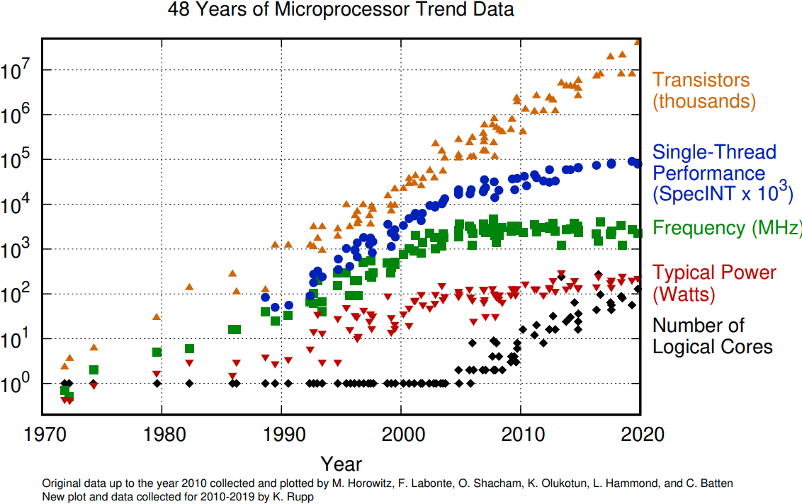
The evolution of microprocessors. The number of transistors per chip increase every 2 years or so. However it can no longer be explored by the core frequency due to power consumption limits. Before 2000, the increase in the single core clock frequency was the major source of the increase in the performance. Mid 2000 mark a transition towards multi-core processors.

Achieving performance has been based on two main strategies over the years:

• Increase the single processor performance:

• More recently, increase the number of physical cores.

Why use GPUs?

The Graphics Processing Unit (GPU) have been the most common accelerators during the last few years. The term GPU sometimes is used interchangeably with the term accelerator. GPU provides much higher instruction throughput and memory bandwidth than CPU within a similar price and power envelope.

How do GPUs differ from CPUs?

CPUs and GPUs were designed with different goals in mind. While the CPU is designed to excel at executing a sequence of operations, called a thread, as fast as possible and can execute a few tens of these threads in parallel, the GPU is designed to excel at executing many thousands of them in parallel. GPUs were initially developed for highly-parallel task of graphic processing and therefore designed such that more transistors are devoted to data processing rather than data caching and flow control. More transistors dedicated to data processing is beneficial for highly parallel computations; the GPU can hide memory access latencies with computation, instead of relying on large data caches and complex flow control to avoid long memory access latencies, both of which are expensive in terms of transistors.

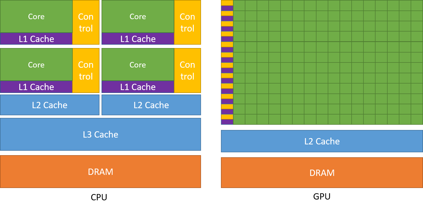
A comparison of the CPU and GPU architecture. CPU (left) has complex core structure and pack several cores on a single chip. GPU cores are very simple in comparison, they also share data and control between each other. This allows to pack more cores on a single chip, thus achieving very hich compute density.

CPU	GPU
General purpose	Highly specialized for parallelism
Good for serial processing	Good for parallel processing
Great for task parallelism	Great for data parallelism
Low latency per thread	High-throughput
Large area dedicated cache and control	Hundreds of floating-point execution units

Summary

• GPUs are highly parallel devices that can execute certain parts of the program in many parallel threads.

• CPU controls the works flow and makes all the allocations and data transfers.

• In order to use the GPU efficiently, one has to split their the problem in many parts that can run simultaneously.

Python on GPU

There has been a lot of progress on Pyhton using GPUs, it is still evolving. There are a couple of options available to work with GPU, but none of them is perfect.

Note

CUDA is the programming model developed by NVIDIA to work with GPU

CuPy

CuPy is a NumPy/SciPy-compatible data array library used on GPU. CuPy has a highly compatible interface with NumPy and SciPy, As stated on its official website, “All you need to do is just replace numpy and scipy with cupy and cupyx.scipy in your Python code.” If you know NumPy, CuPy is a very easy way to get started on the GPU.

cuDF

RAPIDS is a high level packages collections which implement CUDA functionalities and API with Python bindings. cuDF belongs to RAPIDS and is the library for manipulating data frames on GPU. cuDF provides a pandas-like API, so if you are familiar with Pandas, you can accelerate your work without knowing too much CUDA programming.

PyCUDA

PyCUDA is a Python programming environment for CUDA. It allows users to access to NVIDIA’s CUDA API from Python. PyCUDA is powerful library but only runs on NVIDIA GPUs. Knowledge of CUDA programming is needed.

Numba

Same as for CPU, Numba allows users to JIT compile Python code to work on GPU as well. This workshop will focus on Numba only.

Numba for GPUs

Terminology

Numba supports GPUs from both Nvidia and AMD, but we will use terminology from Nvidia as examples in the rest of the course.

Several important terms in the topic of GPU programming are listed here:

• host: the CPU

• device: the GPU

• host memory: the system main memory of the CPU

• device memory: GPU onboard memory

• kernels: a GPU function launched by the host and executed on the device

• device function: a GPU function executed on the device which can only be called from the device (i.e. from a kernel or another device function)

Numba supports GPU programming by directly compiling a restricted subset of Python code into kernels and device functions following the execution model. Kernels written in Numba appear to have direct access to NumPy arrays. NumPy arrays are transferred between the CPU and the GPU automatically.

Note

Kernel declaration

A kernel function is a GPU function that is meant to be called from CPU code. It contains two fundamental characteristics:

• kernels cannot explicitly return a value; all result data must be written to an array passed to the function (if computing a scalar, you will probably pass a one-element array);

• kernels explicitly declare their thread hierarchy when called: i.e. the number of thread blocks and the number of threads per block (note that while a kernel is compiled once, it can be called multiple times with different block sizes or grid sizes).

• Newer GPU devices from NVIDIA support device-side kernel launching; this feature is called dynamic parallelism but Numba does not support it currently

ufunc (gufunc) decorator

Using ufuncs (and generalized ufuncs) is the easist way to run on a GPU with Numba, and it requires minimal understanding of GPU programming. Numba @vectorize will produce a ufunc-like object. This object is a close analog but not fully compatible with a regular NumPy ufunc. Generating a ufunc for GPU requires the explicit type signature and target attribute.

Demo: Numba ufunc

Let’s revisit our example during the episode of optimization.

pythonNumba ufunc cpuNumba ufunc gpu

import math

def f(x,y):
    return math.pow(x,3.0) + 4*math.sin(y)

Let’s benchmark

pythonNumba cpuNumba gpu

import numpy as np
x = np.random.rand(10000000)
res = np.random.rand(10000000)

%%timeit -r 1
for i in range(10000000):
    res[i]=f(x[i], x[i])
# 6.75 s ± 0 ns per loop (mean ± std. dev. of 1 run, 1 loop each)

Numba @vectroize is limited to scalar arguments in the core function, for multi-dimensional arrays arguments, @guvectorize is used. Consider the following example which does matrix multiplication.

Warning

You should never implement such things like matrix multiplication by yourself, there are plenty of existing libraries available.

Demo: Numba gufunc

pythonnumba gufunc cpunumba gufunc gpu

import numpy as np

def matmul_cpu(A,B,C):
    for i in range(A.shape[0]):
        for j in range(B.shape[1]):
            tmp=0.0
            for k in range(B.shape[0]):
                tmp += A[i, k] * B[k, j]
            C[i,j] += tmp

benchmark

Numba gufunc cpuNumba gufunc gpu

import numpy as np
import numba
N = 50
A = np.random.rand(N,N)
B = np.random.rand(N,N)
C = np.random.rand(N,N)
%timeit matmul_numba_cpu(A,B,C)

Note

Numba automatically did a lot of things for us:

• Memory was allocated on GPU

• Data was copied from CPU and GPU

• The kernel was configured and launched

• Data was copied back from GPU to CPU

Alough it is simple to use ufuncs(gfuncs) to run on GPU, the performance is the price we have to pay. In addition, not all functions can be written as ufuncs in practice. To have much more flexibility, one needs to write a kernel on GPU or device function, which requires more understanding of the GPU programming.

GPU Programming Model

Accelerators are a separate main circuit board with the processor, memory, power management, etc., but they can not operate by themselves. They are always part of a system (host) in which the CPUs run the operating systems and control the programs execution. This is reflected in the programming model. CPU (host) and GPU (device) codes are mixed. CPU acts as a main processor, controlling the execution workflow. The host makes all calls, allocates the memory, and handles the memory transfers between CPU and GPU. GPUs run tens of thousands of threads simultaneously on thousands of cores and does not do much of the data management. The device code is executed by doing calls to functions (kernels) written specifically to take advantage of the GPU. The kernel calls are asynchronous, the control is returned to the host after a kernel calls. All kernels are executed sequentially.

GPU Autopsy. Volta GPU

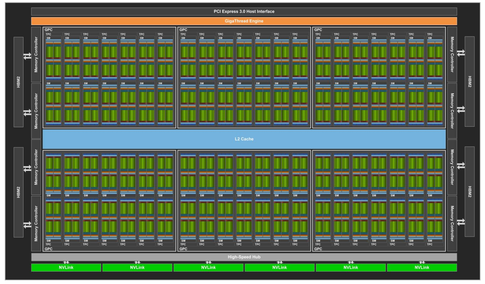
A scheme of NVIDIA Volta GPU.

The NVIDIA GPU architecture is built upon a number of multithreaded Streaming Multiprocessors (SMs), each SM contains a number of compute units. NVIDIA Volta GPU has 80 SMs.

NVIDIA Volta streaming multiprocessor (SM):

• 64 single precision cores

• 32 double precision cores

• 64 integer cores

• 8 Tensore cores

• 128 KB memory block for L1 and shared memory

  • 0 - 96 KB can be set to user managed shared memory

  • The rest is L1

• 65536 registers - enables the GPU to run a very large number of threads

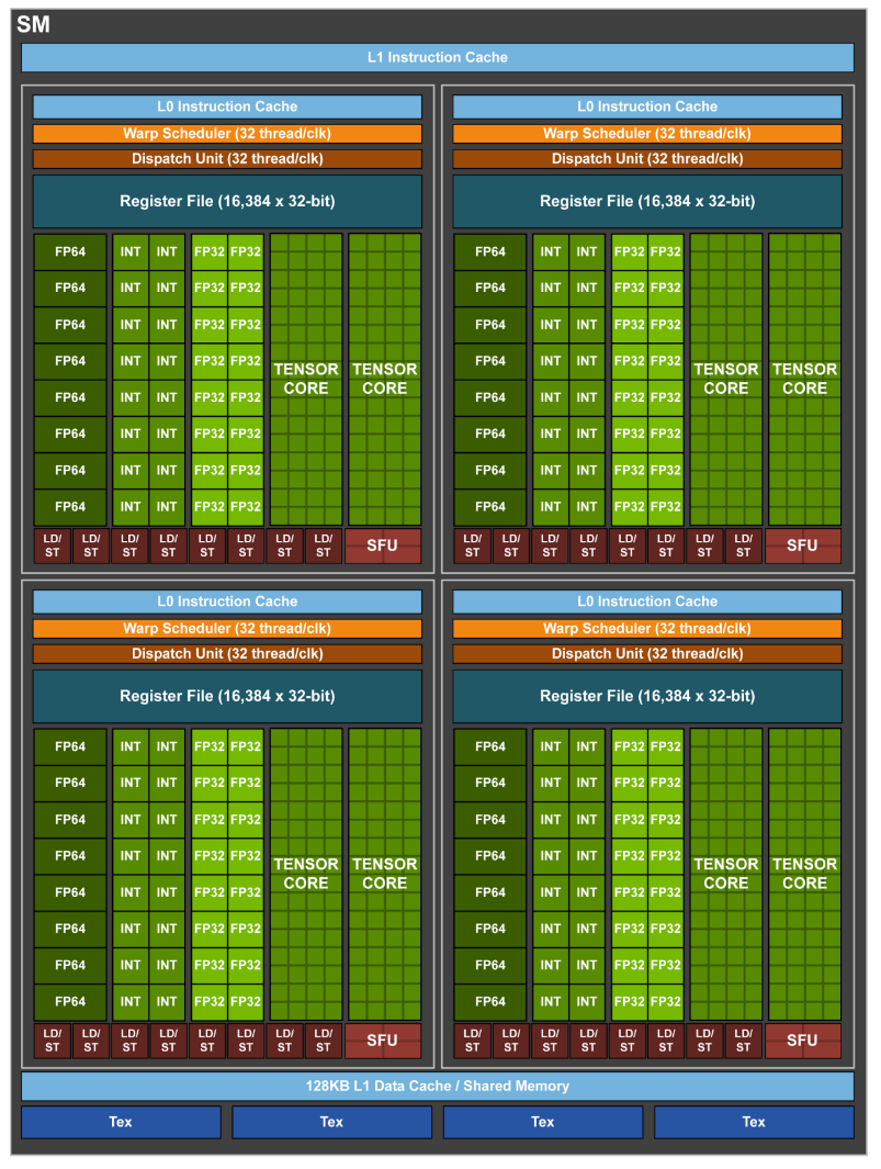
A scheme of NVIDIA Volta streaming multiprocessor.

Thread hierarchy

In order to take advantage of the accelerators it is needed to use parallelism. When a kernel is launched, tens of thousands of threads are created. All threads execute the given kernel with each thread executing the same instructions but on different data (Single Iinstruction Multiple Data parallel programming model). It is therefore crucial to know which thread operates on which array element(s).

In order to know the thread positioning, we need some information about the hierarchy on a software level. When CPU invokes a kernel, all the threads launched in the given kernel are partitioned/grouped into the so-called thread blocks and multiple blocks are combined to form a grid. The thread blocks of the grid are enumerated and distributed to SMs with available execution capacity. Thread blocks are required to execute independently, i.e. it must be possible to execute them in any order: in parallel or in series. In other words, each thread block can be scheduled on any of the available SM within a GPU, in any order, concurrently or sequentially, so that they can be executed on any number of SMs. Because of the design, a GPU with more SMs will automatically execute the program in less time than a GPU with fewer SMs. However, a thread block can not be splitted among the SMs, but in a SM several blocks can be active at any given moment. As thread blocks terminate, new blocks are launched on the vacated SMs. Within a thread block, the threads execute concurrently on the same SM, and they can exchange data via the so called shared memory and can be explicitly synchronized. The blocks can not interact with other blocks.

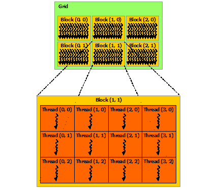
Threads can be identified using a one-dimensional, two-dimensional, or three-dimensional thread index through the buit-in numba.cuda.threadIdx variable, and this provides a natural way to invoke computation across the elements in a domain such as a vector, matrix, or volume. Each block within the grid can be identified by a one-dimensional, two-dimensional, or three-dimensional unique index accessible within the kernel through the built-in numba.cuda.blockIdx variable. The dimension of the thread block is accessible within the kernel through the built-in numba.cuda.blockDim variable. The global index of a thread should be computed from its in-block index, the index of execution block and the block size. For 1D, it is numba.cuda.threadIdx.x + numba.cuda.blockIdx.x * numba.cuda.blockDim.x.

Note

Compared to an one-dimensional declarations of equivalent sizes, using multi-dimensional blocks does not change anything to the efficiency or behaviour of generated code, but can help you write your code in a more natural way.

numba.cuda.threadIdx, numba.cuda.blockIdx and numba.cuda.blockDim are special objects provided by the CUDA backend for the sole purpose of knowing the geometry of the thread hierarchy and the position of the current thread within that geometry. These objects can be 1D, 2D or 3D, depending on how the kernel was invoked. To access the value at each dimension, use the x, y and z attributes of these objects, respectively.

Numba provides simple solution to calculate thread position by calling numba.cuda.grid(ndim) where ndim is the number of dimensions declared when invoking the kernel.

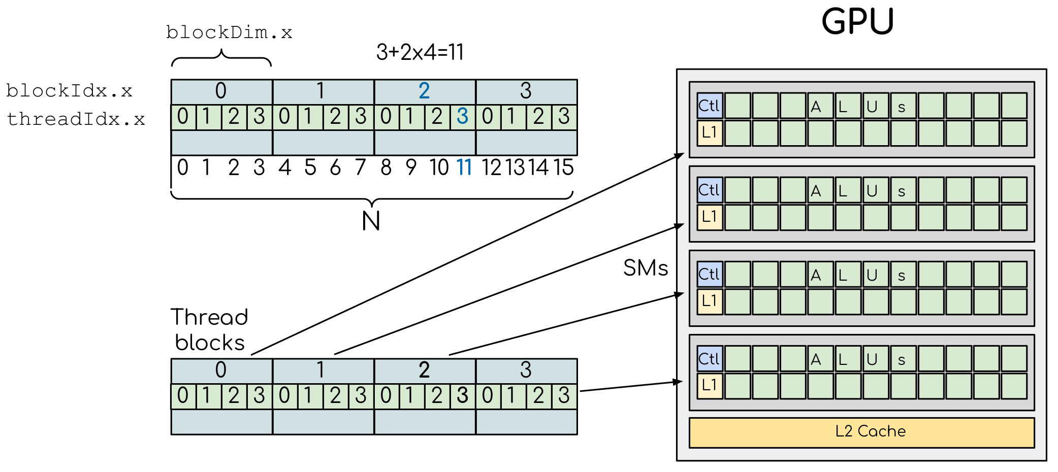
A simple example of the division of threads (green squares) in blocks (cyan rectangles). The equally-sized blocks contain four threads each. The thread index starts from zero in each block. Hence the “global” thread index should be computed from the thread index, block index and block size. This is explained for the thread #3 in block #2 (blue numbers). The thread blocks are mapped to SMs for execution, with all threads within a block executing on the same device. The number of threads within one block does not have to be equal to the number of execution units within multiprocessor. In fact, GPUs can switch between software threads very efficiently, putting threads that currently wait for the data on hold and releasing the resources for threads that are ready for computations. For efficient GPU utilization, the number of threads per block has to be couple of factors higher than the number of computing units on the multiprocessor. Same is true for the number of thread blocks, which can and should be higher than the number of available multiprocessor in order to use the GPU computational resources efficiently.

It is important to notice that the total number of threads in a grid is a multiple of the block size. This is not necessary the case for the problem that we are solving: the length of the vectors can be non-divisible by selected block size. So we either need to make sure that the threads with index large than the size of the vector don’t do anything, or add padding to the vectors. The former is a simple solution, i.e. by adding a condition after the global thread index is computed.

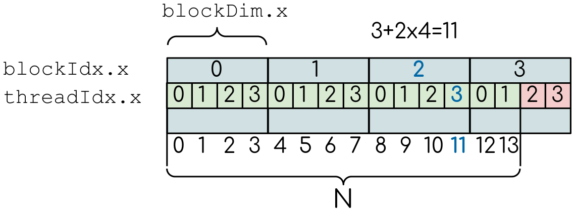
The total number of threads that are needed for the execution (N) can often not be a multiple of the block size and some of the threads will be idling or producing unused data (red blocks).

Note

Unless you are really sure that the block size and grid size are a divisor of your array size, you must check boundaries.

To obtain the best choice of the thread grid is not a simple task, since it depends on the specific implemented algorithm and GPU computing capability. The total number of threads is equal to the number of threads per block times the number of blocks per grid. The number of thread blocks per grid is usually dictated by the size of the data being processed, and it should be large enough to fully utilize the GPU.

• start with 20-100 blocks, the number of blocks is usually chosen to be 2x-4x the number of SMs

• the CUDA kernel launch overhead does depend on the number of blocks, so we find it best not to launch with very large number of blocks

The size of the number of threads per block should be a multiple of 32, values like 128, 256 or 512 are frequently used

• it should be lower than 1024 since it determines how many threads share a limited size of the shared memory

• it must be large than the number of available (single precision, double precision or integer operation) cores in a SM to fully occupy the SM

Data and Memory management

With many cores trying to access the memory simultaneously and with little cache available, the accelerator can run out of memory very quickly. This makes the data and memory management an essential task on the GPU.

Data transfer

Although Numba could transfer data automatically from/to the device, these data transfers are slow, sometimes even more than the actual on-device computation. Therefore explicitly transfering the data is necessary and should be minimised in real applications.

Using numba.cuda functions, one can transfer data from/to device. To transfer data from cpu to gpu, one could use to_device() method:

d_x = numba.cuda.to_device(x)
d_y = numba.cuda.to_device(y)

the resulting d_x is a DeviceNDArray. To transfer data on the device back to the host, one can use the copy_to_host() method:

d_x.copy_to_host(h_x)
h_y = d_y.copy_to_host()

Memory hierarchy

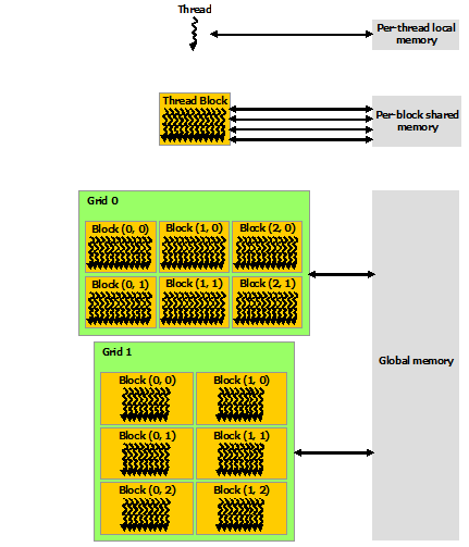
As shown in the figure, CUDA threads may access data from different memory spaces during kernel execution:

• local memory: Each thread has private local memory.

• shared memory: Each thread block has shared memory visible to all threads of the thread block and with the same lifetime as the block.

• global memory: All threads have access to the same global memory.

Both local and global memory resides in device memory, so memory accesses have high latency and low bandwidth, i.e. slow access time. On the other hand, shared memory has much higher bandwidth and much lower latency than local or global memory. However, only a limited amount of shared memory can be allocated on the device for better performance. One can think it as a manually-managed data cache.

CUDA JIT decorator

CUDA Kernel and device functions are created with the numba.cuda.jit decorator on Nvidia GPUs. We will use Numba function numba.cuda.grid(ndim) to calculate the global thread positions.

Demo: CUDA kernel

ufunc gpuCUDA kernel

import math
import numba

@numba.vectorize([numba.float64(numba.float64, numba.float64)], target='cuda')
def f_numba_gpu(x,y):
    return math.pow(x,3.0) + 4*math.sin(y)

benchmark

CUDA kernelCUDA kernel without data transfer

import numpy as np
import math
import numba
a = np.random.rand(10000000)
b = np.random.rand(10000000)
c = np.random.rand(10000000)
threadsperblock = 32
blockspergrid = 256
%timeit math_kernel[threadsperblock, blockspergrid](a, b, c); numba.cuda.synchronize()
# 103 ms ± 616 µs per loop (mean ± std. dev. of 7 runs, 10 loops each)

Demo: CUDA kernel matrix multiplication

gufunc gpuCUDA kernel

import numpy as np
import numba

#@numba.guvectorize(['(float64[:,:], float64[:,:], float64[:,:])'], '(m,l),(l,n)->(m,n)', target='cuda')
@numba.guvectorize([numba.void(numba.float64[:,:], numba.float64[:,:], numba.float64[:,:])], '(m,l),(l,n)->(m,n)', target='cuda')
def matmul_numba_gpu(A,B,C):
    for i in range(A.shape[0]):
        for j in range(B.shape[1]):
            tmp=0.0
            for k in range(B.shape[0]):
                tmp += A[i, k] * B[k, j]
            C[i,j] += tmp

Benchmark:

NumPygufunc gpuCUDA kernelCUDA kernel without data transfer

import numpy as np
    N = 50
    A = np.random.rand(N,N)
    B = np.random.rand(N,N)
    C = np.random.rand(N,N)
    %timeit C=np.matmul(A,B)
# 4.65 µs ± 45.9 ns per loop (mean ± std. dev. of 7 runs, 100,000 loops each)

Note

numba.cuda.synchronize() is used after the kernel launch to make sure the profiling is correct.

There are times when the gufunc kernel uses too many of a GPU’s resources, which can cause the kernel launch to fail. The user can explicitly control the maximum size of the thread block by setting the max_blocksize attribute on the compiled gufunc object. e.g. matmul_numba_gpu.max_blocksize = 32

Optimization

GPU can be easily misused and which leads to a low performance. One should condiser the following points when programming with GPU:

• Maximize GPU utilization

  • input data size to keep GPU busy

  • high arithmetic intensity

• Maximize memory throughput

  • minimizing data transfers between the host and the device

  • minimizing redundant data accesses to global memory by using shared memory and cache

• Maximize instruction throughput

  • Asynchronous execution

  • data types: 64bit data types (integer and floating point) have a significant cost when running on GPU compared to 32bit.

Asynchronous execution

Although the evaluation of computation heavy kernels is noticeable quicker on a GPU, we still have some room for improvement. A typical GPU program that does not explore the task-based parallelism executed sequentially is shown on the figure below:

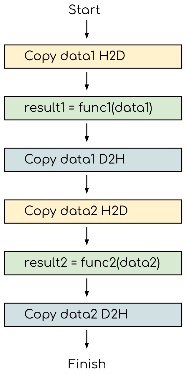
All the data transfers and two functions are executed sequentially.

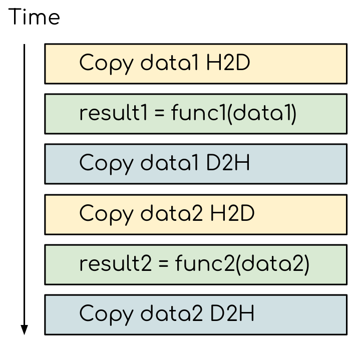
As a result, the execution timeline looks similar to this:

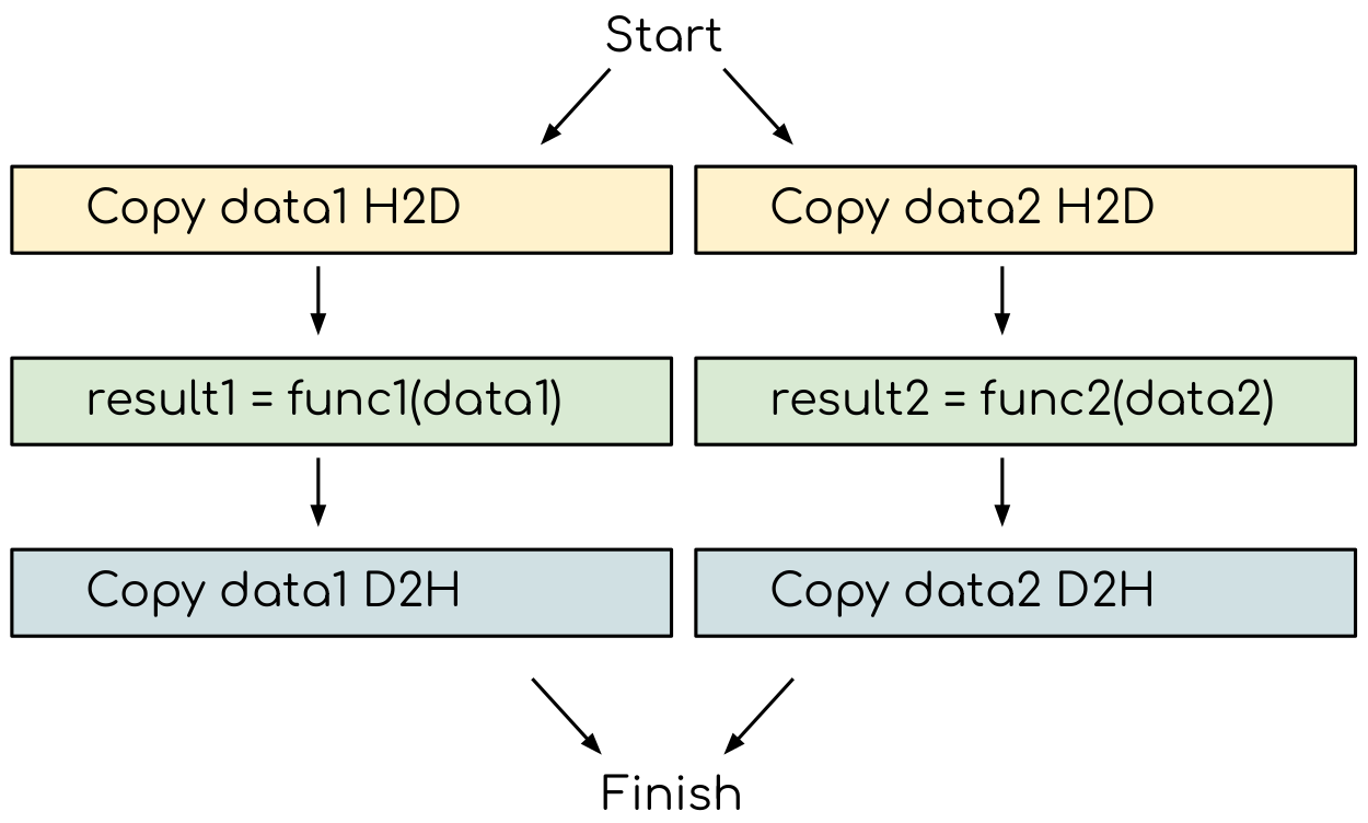
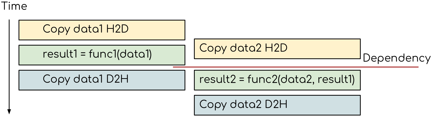
On a GPU, the host to device copy, kernel evaluation and device to host copy require different resources. Hence, while the data is being copied, GPU can execute the computational kernel without interfering with the data copying. To explore the task-based parallelism, we would like to execute the program as below:

and the resulting execution timeline looks similar to this:

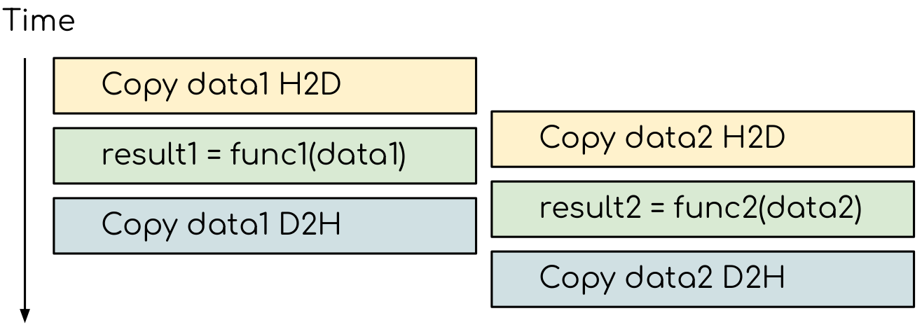
The execution timeline of the asynchronous GPU program. The different tasks will overlap to each other to a certain extent that they do not interfere with each other. Note that there are still dependencies between tasks: we can not run the func1(..) before the data1 is on the GPU and we can not copy the result1 to the CPU before the kernel is finished. In order to express such sequential dependencies, asynchronous executions are used. Tasks that are independent can run simultaneously.

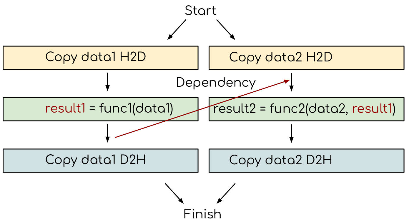
Adding extra dependency between two tasks.

Let us look at one step further by adding extra dependency between two tasks. Assume that the func2(..) now needs the result of the func1(..) to be evaluated. This is easy to do in the program.

Adding extra dependency between two tasks.

Exercises

Perform matrix multiplication with single precision

In this exercise, we will compare the performance by using different precisions. We will run the matrix multiplication CUDA kernel i.e. matmul_kernel using input data with double and single precisions. Depending on what generation of GPU you are running on, the performance can be quite different.

One can find more information about different Nvidia GPUs’ throughputs of the arithmetic instructions here

Interactive modeBatch mode

import numpy as np
import numba
import numba.cuda

@numba.cuda.jit
def matmul_kernel(A, B, C):
    i, j = numba.cuda.grid(2)
    if i < C.shape[0] and j < C.shape[1]:
        tmp = 0.
        for k in range(A.shape[1]):
            tmp += A[i, k] * B[k, j]
        C[i, j] = tmp

# Benchmark

# first generate double precision input data

N = 8192
A = np.random.rand(N,N)
B = np.random.rand(N,N)
C = np.random.rand(N,N)

# copy them to GPU

d_A = numba.cuda.to_device(A)
d_B = numba.cuda.to_device(B)
d_C = numba.cuda.to_device(C)

# setup grid and block

threadsperblock = (16, 16)
blockspergrid = (10,10)

# benchmark double precision input data

%timeit matmul_kernel[blockspergrid, threadsperblock](d_A, d_B, d_C); numba.cuda.synchronize()

# then generate single precision input data

d_A32 = numba.cuda.to_device(A.astype(np.float32))
d_B32 = numba.cuda.to_device(B.astype(np.float32))
d_C32 = numba.cuda.to_device(C.astype(np.float32))

# benchmark single precision input data

%timeit matmul_kernel[blockspergrid, threadsperblock](d_A32, d_B32, d_C32); numba.cuda.synchronize()

TEST USING BATCH MODE!!!

#!/bin/bash
#SBATCH --job-name="test"
#SBATCH --time=00:10:00
#SBATCH --nodes=1
#SBATCH --gres=gpu:1
#SBATCH --ntasks-per-core=1
#SBATCH --ntasks-per-node=1
#SBATCH --cpus-per-task=1
#SBATCH --partition=gpu
#SBATCH --mem=4GB
#SBATCH --account=d2021-135-users
#SBATCH --reservation=ENCCS-HPDA-Workshop

module add Anaconda3/2020.11
#conda activate pyhpda
conda activate /ceph/hpc/home/euqiamgl/.conda/envs/pyhpda

python $1 > $1.out

exit 0

• Save the solution in a Python script called sbatch_matmul_dtype.py

• Save the above template file job.sh in the same folder as sbatch_matmul_dtype.py

• Submit the job by following the instructions below

• The output will be written in sbatch_matmul_dtype.py.out

# go to the directory where the files job.sh and sbatch_matmul_dtype.py are
$ cd /path/to/somewhere
$ sbatch job.sh sbatch_matmul_dtype.py

Perform matrix multiplication with shared memory

We will start from one implementation of the square matrix multiplication using shared memory. This implementation is taken from Numba official document, however there is arguably at least one error in it. Try to find where the error is and fix it:

import numba

TPB = 16
@numba.cuda.jit
def matmul_sm(A, B, C):
    # Define an array in the shared memory
    # The size and type of the arrays must be known at compile time
    sA = numba.cuda.shared.array(shape=(TPB, TPB), dtype=numba.float64)
    sB = numba.cuda.shared.array(shape=(TPB, TPB), dtype=numba.float64)

    x, y = numba.cuda.grid(2)

    tx = numba.cuda.threadIdx.x
    ty = numba.cuda.threadIdx.y
    bpg = numba.cuda.gridDim.x    # blocks per grid

    if x >= C.shape[0] and y >= C.shape[1]:
        return

    tmp = 0.
    for i in range(bpg):
        sA[tx, ty] = A[x, ty + i * TPB]
        sB[tx, ty] = B[tx + i * TPB, y]
        # Wait until all threads finish preloading
        numba.cuda.syncthreads()

        for j in range(TPB):
            tmp += sA[tx, j] * sB[j, ty]

        # Wait until all threads finish computing
        numba.cuda.syncthreads()

    C[x, y] = tmp

Hint

• data range check: we require neither x nor y is out of range. The and should have been an or.

• numba.cuda.syncthreads() in conditional code: __syncthreads() is allowed in conditional code but only if the conditional evaluates identically across the entire thread block, otherwise the code execution is likely to hang or produce unintended side effects.

Solution

import numba

TPB = 16
@numba.cuda.jit
def matmul_sm(A, B, C):
    # Define an array in the shared memory
    # The size and type of the arrays must be known at compile time
    sA = numba.cuda.shared.array(shape=(TPB, TPB), dtype=numba.float64)
    sB = numba.cuda.shared.array(shape=(TPB, TPB), dtype=numba.float64)

    x, y = numba.cuda.grid(2)

    tx = numba.cuda.threadIdx.x
    ty = numba.cuda.threadIdx.y
    bpg = numba.cuda.gridDim.x    # blocks per grid

    # Each thread computes one element in the result matrix.
    # The dot product is chunked into dot products of TPB-long vectors.
    tmp = 0.
    for i in range(bpg):
        # Preload data into shared memory
        sA[tx, ty] = 0
        sB[tx, ty] = 0
        if x < A.shape[0] and (ty+i*TPB) < A.shape[1]:
          sA[tx, ty] = A[x, ty + i * TPB]
        if y < B.shape[1] and (tx+i*TPB) < B.shape[0]:
          sB[tx, ty] = B[tx + i * TPB, y]

        # Wait until all threads finish preloading
        numba.cuda.syncthreads()

        # Computes partial product on the shared memory
        for j in range(TPB):
            tmp += sA[tx, j] * sB[j, ty]

        # Wait until all threads finish computing
        numba.cuda.syncthreads()
    if x < C.shape[0] and y < C.shape[1]:
        C[x, y] = tmp

Benchmark

import numpy as np
import numba
import numba.cuda
import time

N = 8192
A = np.random.rand(N,N)
B = np.random.rand(N,N)
C = np.random.rand(N,N)

d_A = numba.cuda.to_device(A)
d_B = numba.cuda.to_device(B)
d_C = numba.cuda.to_device(C)

threadsperblock = (16, 16)
blockspergrid = (10,10)

n_loop=20
test3=np.empty(n_loop)

for i in range(n_loop):
    t_s=time.time()
    matmul_sm[blockspergrid, threadsperblock](d_A, d_B, d_C); numba.cuda.synchronize()
    t_e=time.time()
    test3[i]=t_e - t_s


record = test3
print("matmul_sm Runtime")
print("average {:.5f} second (except 1st run)".format(record[1:].mean()))

RUN THIS!!!

• Save the solution and add benchmark part as well in a Python script called sbatch_matmul_sm.py

• Copy or download job.sh to the same folder as sbatch_matmul_sm.py

• Submit the job by following the instructions below

• The output will be written in sbatch_matmul_sm.py.out

# go to the directory where job.sh and sbatch_matmul_sm.py are
$ cd /path/to/somewhere
$ sbatch job.sh sbatch_matmul_sm.py

Discrete Laplace Operator

In this exercise, we will work with the discrete Laplace operator. It has a wide applications including numerical analysis, physics problems, image processing and machine learning as well. Here we consider a simple two-dimensional implementation with finite-difference formula i.e. the five-point stencil, which reads:

\[u_{out}(i,j) = 0.25*[ u(i-1,j) + u(i+1,j) + u(i,j-1) + u(i,j+1) ]\]

where \(u(i,j)\) refers to the input at location with integer index \(i\) and \(j\) within the domain.

You will start with a naive implementation in Python and you should optimize it to run on both CPU and GPU using what we learned so far.

The Laplace codeBenchmark

def lap2d(u, unew):
    M, N = u.shape     
    for i in range(1, M-1):
        for j in range(1, N-1):             
            unew[i, j] = 0.25 * ( u[i+1, j] + u[i-1, j] + u[i, j+1] + u[i, j-1] )

Solution

Optimization on CPU

numpynumba gufuncnumba JIT

def lap2d_numpy(u, unew):
    unew[1:-1,1:-1]=0.25*(u[:-2,1:-1]+u[2:,1:-1]+u[1:-1,:-2]+u[1:-1,2:])          


# Benchmark

import numpy as np

M = 4096
N = 4096

u = np.zeros((M, N), dtype=np.float64)
unew = np.zeros((M, N), dtype=np.float64)

%timeit lap2d_numpy(u, unew)

Optimization on GPU

numba gufuncnumba CUDA kernelRUN THIS!!!

import numpy as np
import numba

@numba.guvectorize(['void(float64[:,:],float64[:,:])'],'(m,n)->(m,n)',target='cuda')
def lap2d_numba_gu_gpu(u, unew):
    M, N = u.shape   
    for i in range(1, M-1):
        for j in range(1, N-1):  
            unew[i, j] = 0.25 * ( u[i+1, j] + u[i-1, j] + u[i, j+1] + u[i, j-1] )   


# Benchmark

M = 4096
N = 4096

u = np.zeros((M, N), dtype=np.float64)
unew = np.zeros((M, N), dtype=np.float64)

%timeit lap2d_numba_gu_gpu(u, unew)

Keypoints

• Numba gufuncs are easy to use on GPU

• Always consider input data size, compute complexity, host/device data copy and data type when programing with GPU