Dask for Scalable Analytics
Objectives
Understand how Dask achieves parallelism
Learn a few common workflows with Dask
Understand lazy execution
Instructor note
40 min teaching/type-along
40 min exercises
Overview
An increasingly common problem faced by researchers and data scientists today is that datasets are becoming larger and larger and modern data analysis is thus becoming more and more computationally demanding. The first difficulty to deal with is when the volume of data exceeds one’s computer’s RAM. Modern laptops/desktops have about 10 GB of RAM. Beyond this threshold, some special care is required to carry out data analysis. The next threshold of difficulty is when the data can not even fit on the hard drive, which is about a couple of TB on a modern laptop. In this situation, it is better to use an HPC system or a cloud-based solution, and Dask is a tool that helps us easily extend our familiar data analysis tools to work with big data. In addition, Dask can also speeds up our analysis by using multiple CPU cores which makes our work run faster on laptop, HPC and cloud platforms.
What is Dask?
Dask is composed of two parts:
Dynamic task scheduling optimized for computation. Similar to other workflow management systems, but optimized for interactive computational workloads.
“Big Data” collections like parallel arrays, dataframes, and lists that extend common interfaces like NumPy, Pandas, or Python iterators to larger-than-memory or distributed environments. These parallel collections run on top of dynamic task schedulers.

High level collections are used to generate task graphs which can be executed by schedulers on a single machine or a cluster. From the Dask documentation.
Dask clusters
Dask needs computing resources in order to perform parallel computations. “Dask Clusters” have different names corresponding to different computing environments, for example:
LocalCluster on laptop/desktop/cluster
PBSCluster or SLURMCluster on HPC
Kubernetes cluster in the cloud
Each cluster will be allocated with a given number of “workers” associated with CPU and RAM and the Dask scheduling system automatically maps jobs to each worker.
Dask provides four different schedulers:
Type |
Multi-node |
Description |
|
No |
A single-machine scheduler backed by a thread pool |
|
No |
A single-machine scheduler backed by a process pool |
|
No |
A single-threaded scheduler, used for debugging |
|
yes |
A distributed scheduler for executing on multiple nodes/machines |
Here we will focus on using a LocalCluster, and it is recommended to use
a distributed scheduler dask.distributed. It is more sophisticated, offers more features,
but requires minimum effort to set up. It can run locally on a laptop and scale up to a cluster.
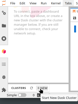
Alternative 1: Initializing a Dask LocalCluster via JupyterLab
This makes use of the dask-labextension which is pre-installed in our conda environment.
Start New Dask Cluster from the sidebar and by clicking on
+ NEWbutton.Click on the
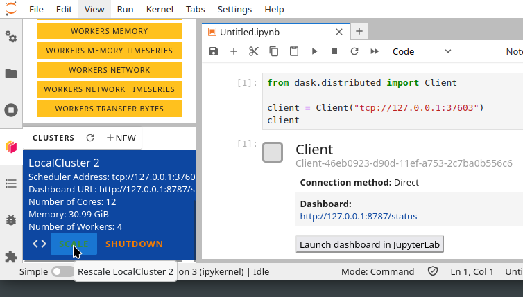
< >button to inject the client code into a notebook cell. Execute it.
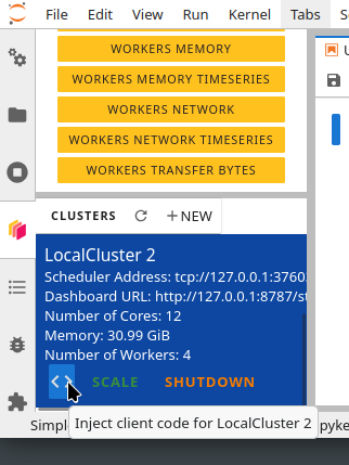
You can scale the cluster for more resources or launch the dashboard.
Alternative 2: We can also start a LocalCluster scheduler manually, which makes use of:
all the cores and RAM we have on the machine by:
from dask.distributed import Client, LocalCluster
# create a local cluster
cluster = LocalCluster()
# connect to the cluster we just created
client = Client(cluster)
client
Or you can simply lauch a Client() call which is shorthand for what is described above.
from dask.distributed import Client
client = Client() # same as Client(processes=True)
client
which limits the compute resources available as follows:
from dask.distributed import Client, LocalCluster

cluster = LocalCluster(
   n_workers=4,
   threads_per_worker=1,
   memory_limit='4GiB'  # memory limit per worker
)
client = Client(cluster)
client
Note
When setting up the cluster, one should consider the balance between the number of workers
and threads per worker with different workloads by setting the parameter processes.
By default processes=True and this is a good choice for workloads that have the GIL,
thus it is better to have more workers and fewer threads per worker. Otherwise, when processes=False,
in this case all workers run as threads within the same process as the client,
and they share memory resources. This works well for large datasets.
Cluster managers also provide useful utilities: for example if a cluster manager supports scaling, you can modify the number of workers manually or automatically based on workload:
cluster.scale(10)  # Sets the number of workers to 10
cluster.adapt(minimum=1, maximum=10)  # Allows the cluster to auto scale to 10 when tasks are computed
Dask distributed scheduler also provides live feedback via its interactive dashboard. A link that redirects to the dashboard will prompt in the terminal where the scheduler is created, and it is also shown when you create a Client and connect the scheduler. By default, when starting a scheduler on your local machine the dashboard will be served at http://localhost:8787/status and can be always queried from commond line by:
cluster.dashboard_link
http://127.0.0.1:8787/status
# or
client.dashboard_link
When everything finishes, you can shut down the connected scheduler and workers
by calling the shutdown() method:
client.shutdown()
Dask collections
Dask provides dynamic parallel task scheduling and three main high-level collections:
dask.array: Parallel NumPy arrays
dask.dataframe: Parallel Pandas DataFrames
dask.bag: Parallel Python Lists
Dask arrays
A Dask array looks and feels a lot like a NumPy array. However, a Dask array uses the so-called “lazy” execution mode, which allows one to build up complex, large calculations symbolically before turning them over the scheduler for execution.
Lazy evaluation
Contrary to normal computation, lazy execution mode is when all the computations needed to generate results are symbolically represented, forming a queue of tasks mapped over data blocks. Nothing is actually computed until the actual numerical values are needed, e.g. plotting, to print results to the screen or write to disk. At that point, data is loaded into memory and computation proceeds in a streaming fashion, block-by-block. The actual computation is controlled by a multi-processing or thread pool, which allows Dask to take full advantage of multiple processors available on the computers.
import numpy as np
shape = (1000, 4000)
ones_np = np.ones(shape)
ones_np
ones_np.nbytes / 1e6
Now let’s create the same array using Dask’s array interface.
import dask.array as da
shape = (1000, 4000)
ones = da.ones(shape)
ones
Although this works, it is not optimized for parallel computation. In order to use all
available computing resources, we also specify the chunks argument with Dask,
which describes how the array is split up into sub-arrays:
import dask.array as da
shape = (1000, 4000)
chunk_shape = (1000, 1000)
ones = da.ones(shape, chunks=chunk_shape)
ones
Note
In this course, we will use a chunk shape, but other ways to specify chunks size can be found here
https://docs.dask.org/en/stable/array-chunks.html#specifying-chunk-shapes
Let us further calculate the sum of the dask array:
sum_da = ones.sum()
So far, only a task graph of the computation is prepared.
We can visualize the task graph by calling visualize():
dask.visualize(sum_da)
# or
sum_da.visualize()
One way to trigger the computation is to call compute():
dask.compute(sum_da)
# or
sum_da.compute()
You can find additional details and examples here https://examples.dask.org/array.html.
Dask dataframe
Dask dataframes split a dataframe into partitions along an index and can be used in situations where one would normally use Pandas, but this fails due to data size or insufficient computational efficiency. Specifically, you can use Dask dataframes to:
manipulate large datasets, even when these don’t fit in memory
accelerate long computations by using many cores
perform distributed computing on large datasets with standard Pandas operations like groupby, join, and time series computations.
Let us revisit the dataset containing the Titanic passenger list, and now transform it to a Dask dataframe:
import pandas as pd
import dask.dataframe as dd

url = "https://raw.githubusercontent.com/pandas-dev/pandas/master/doc/data/titanic.csv"

df = pd.read_csv(url, index_col="Name")
# read a Dask Dataframe from a Pandas Dataframe
ddf = dd.from_pandas(df, npartitions=10)
Alternatively you can directly read into a Dask dataframe, whilst also modifying
how the dataframe is partitioned in terms of blocksize:
# blocksize=None which means a single chunk is used
df = dd.read_csv(url,blocksize=None).set_index('Name')
ddf= df.repartition(npartitions=10)

# blocksize="4MB" or blocksize=4e6
ddf = dd.read_csv(url,blocksize="4MB").set_index('Name')
ddf.npartitions

# blocksize="default" means the chunk is computed based on
# available memory and cores with a maximum of 64MB
ddf = dd.read_csv(url,blocksize="default").set_index('Name')
ddf.npartitions
Dask dataframes do not support the entire interface of Pandas dataframes, but the most commonly used methods are available. For a full listing refer to the dask dataframe API.
We can for example perform the group-by operation we did earlier, but this time in parallel:
# add a column
ddf["Child"] = ddf["Age"] < 12
ddf.groupby(["Sex", "Child"])["Survived"].mean().compute()
However, for a small dataframe like this the overhead of parallelisation will far outweigh the benefit.
You can find additional details and examples here https://examples.dask.org/dataframe.html.
Dask bag
A Dask bag enables processing data that can be represented as a sequence of arbitrary inputs (“messy data”), like in a Python list. Dask Bags are often used to for preprocessing log files, JSON records, or other user defined Python objects.
We will content ourselves with implementing a dask version of the word-count problem, specifically the step where we count words in a text.
Demo: Dask version of word-count
If you have not already cloned or downloaded word-count-hpda repository,
get it from here.
Then, navigate to the word-count-hpda directory. The serial version (wrapped in
multiple functions in the source/wordcount.py code) looks like this:
filename = './data/pg10.txt'
DELIMITERS = ". , ; : ? $ @ ^ < > # % ` ! * - = ( ) [ ] { } / \" '".split()

with open(filename, "r") as input_fd:
    lines = input_fd.read().splitlines()

counts = {}
for line in lines:
    for purge in DELIMITERS:
        line = line.replace(purge, " ")
    words = line.split()
    for word in words:
        word = word.lower().strip()
        if word in counts:
            counts[word] += 1
        else:
            counts[word] = 1

sorted_counts = sorted(
   list(counts.items()),
   key=lambda key_value: key_value[1],
   reverse=True
)

sorted_counts[:10]
A very compact dask.bag version of this code is as follows:
import dask.bag as db
filename = './data/pg10.txt'
DELIMITERS = ". , ; : ? $ @ ^ < > # % ` ! * - = ( ) [ ] { } / \" '".split()

text = db.read_text(filename, blocksize='1MiB')
sorted_counts = (
   text
   .filter(lambda word: word not in DELIMITERS)
   .str.lower()
   .str.strip()
   .str.split()
   .flatten()
   .frequencies().topk(10,key=1)
   .compute()
)

sorted_counts
The last two steps of the pipeline could also have been done with a dataframe:
filtered = (
   text
   .filter(lambda word: word not in DELIMITERS)
   .str.lower()
   .str.strip()
   .str.split()
   .flatten()
)
ddf = filtered.to_dataframe(columns=['words'])
ddf['words'].value_counts().compute()[:10]
When to use Dask
There is no benefit from using Dask on small datasets. But imagine we were analysing a very large text file (all tweets in a year? a genome?). Dask provides both parallelisation and the ability to utilize RAM on multiple machines.
Exercise set 1
Choose an exercise with the data structure that you are most interested in: 1.1. using dask.array, 1.2. using dask.dataframe or 1.3. using dask.bag.
1.1. using dask.array
Chunk size
The following example calculate the mean value of a random generated array. Run the example and see the performance improvement by using dask.
import numpy as np

%%time
x = np.random.random((20000, 20000))
y = x.mean(axis=0)
import dask
import dask.array as da

%%time
x = da.random.random((20000, 20000), chunks=(1000, 1000))
y = x.mean(axis=0)
y.compute()
But what happens if we use different chunk sizes? Try out with different chunk sizes:
What happens if the dask chunks=(20000,20000)
What happens if the dask chunks=(250,250)
Choice of chunk size
The choice is problem dependent, but here are a few things to consider:
Each chunk of data should be small enough so that it fits comforably in each worker’s available memory. Chunk sizes between 10MB-1GB are common, depending on the availability of RAM. Dask will likely manipulate as many chunks in parallel on one machine as you have cores on that machine. So if you have a machine with 10 cores and you choose chunks in the 1GB range, Dask is likely to use at least 10 GB of memory. Additionally, there should be enough chunks available so that each worker always has something to work on.
On the otherhand, you also want to avoid chunk sizes that are too small as we see in the exercise. Every task comes with some overhead which is somewhere between 200us and 1ms. Very large graphs with millions of tasks will lead to overhead being in the range from minutes to hours which is not recommended.
1.2. using dask.dataframe
Benchmarking DataFrame.apply()
Recall the
word count
project that we encountered earlier and the scipy.optimize.curve_fit() function.
The results.csv file contains word counts of the 10
most frequent words in different texts, and we want to fit a power law to the
individual distributions in each row.
Here are our fitting functions:
from scipy.optimize import curve_fit

def powerlaw(x, A, s):
    return A * np.power(x, s)

def fit_powerlaw(row):
    X = np.arange(row.shape[0]) + 1.0
    params, cov = curve_fit(f=powerlaw, xdata=X, ydata=row, p0=[100, -1], bounds=(-np.inf, np.inf))
    return params[1]
Compare the performance of
dask.dataframe.DataFrame.apply() with
pandas.DataFrame.apply()
for the this example. You will probably see a slowdown due to the parallelisation
overhead. But what if you add a time.sleep(0.01) inside fit_powerlaw() to
emulate a time-consuming calculation?
Hints
You will need to call
apply()on the dataframe starting from column 1:dataframe.iloc[:,1:].apply()Remember that both Pandas and Dask have the
read_csv()function.Try repartitioning the dataframe into 4 partitions with
ddf4=ddf.repartition(npartitions=4).You will probably get a warning in your Dask version that You did not provide metadata. To remove the warning, add the
meta=(None, "float64")flag toapply(). For the current data, this does not affect the performance.
More hints with Pandas code
You need to reimplement the highlighted part which creates the
dataframe and applies the fit_powerlaw() function.
import numpy as np
import pandas as pd
from scipy.optimize import curve_fit
import time

def powerlaw(x, A, s):
    return A * np.power(x, s)

def fit_powerlaw(row):
    X = np.arange(row.shape[0]) + 1.0
    params, cov = curve_fit(f=powerlaw, xdata=X, ydata=row, p0=[100, -1], bounds=(-np.inf, np.inf))
    time.sleep(0.01)
    return params[1]


df = pd.read_csv("https://raw.githubusercontent.com/ENCCS/hpda-python/main/content/data/results.csv")
%timeit results = df.iloc[:,1:].apply(fit_powerlaw, axis=1)
Solution
import numpy as np
import dask.dataframe as dd
from scipy.optimize import curve_fit
import time

def powerlaw(x, A, s):
    return A * np.power(x, s)

def fit_powerlaw(row):
    X = np.arange(row.shape[0]) + 1.0
    params, cov = curve_fit(f=powerlaw, xdata=X, ydata=row, p0=[100, -1], bounds=(-np.inf, np.inf))
    time.sleep(0.01)
    return params[1]

ddf = dd.read_csv("https://raw.githubusercontent.com/ENCCS/hpda-python/main/content/data/results.csv")
ddf4=ddf.repartition(npartitions=4)

# Note the optional argument ``meta`` which is recommended for dask dataframes.
# It should contain an empty ``pandas.DataFrame`` or ``pandas.Series``
# that matches the dtypes and column names of the output,
# or a dict of ``{name: dtype}`` or iterable of ``(name, dtype)``.

results = ddf4.iloc[:,1:].apply(fit_powerlaw, axis=1, meta=(None, "float64"))
%timeit results.compute()
results.visualize()
1.3. using dask.bag
Break down the dask.bag computational pipeline
Revisit the
word count problem
and the implementation with a dask.bag that we saw above.
To get a feeling for the computational pipeline, break down the computation into separate steps and investigate intermediate results using
compute().Benchmark the serial and
dask.bagversions. Do you see any speedup? What if you have a larger textfile? You can for example concatenate all texts into a single file:cat data/*.txt > data/all.txt.
Low level interface: delayed
Sometimes problems don’t fit into one of the collections like
dask.array or dask.dataframe, they are not as simple as just a big array or dataframe.
In these cases, dask.delayed may be the right choice. If the problem is paralellisable,
we can use dask.delayed which allows users to make function calls lazy
and thus can be put into a task graph with dependencies.
Consider the following example. The functions are very simple, and they sleep for a prescribed time to simulate real work:
import time

def inc(x):
    time.sleep(0.5)
    return x + 1

def dec(x):
    time.sleep(0.3)
    return x - 1

def add(x, y):
    time.sleep(0.1)
    return x + y
Let us run the example first, one after the other in sequence:
%%timeit
x = inc(1)
y = dec(2)
z = add(x, y)
# 902 ms ± 367 µs per loop (mean ± std. dev. of 7 runs, 1 loop each)
Note that the first two functions inc and dec don’t depend on each other,
we could have called them in parallel. We can call dask.delayed on these functions
to make them lazy and tasks into a graph which we will run later on parallel hardware.
import dask
inc_delay = dask.delayed(inc)
dec_delay = dask.delayed(dec)
add_delay = dask.delayed(add)
%%timeit
x = inc_delay(1)
y = dec_delay(2)
z = add_delay(x, y)
# 59.6 µs ± 356 ns per loop (mean ± std. dev. of 7 runs, 10,000 loops each)
%%timeit
x = inc_delay(1)
y = dec_delay(2)
z = add_delay(x, y)
z.compute()
# 603 ms ± 181 µs per loop (mean ± std. dev. of 7 runs, 1 loop each)
Default scheduler for dask collections
dask.array and dask.dataframe use the threads scheduler
dask.bag uses the processes scheduler
In case to change the default scheduler, using dask.config.set is recommended:
# To set globally
dask.config.set(scheduler='processes')
x.compute()

# To set it as a context manager
with dask.config.set(scheduler='threads'):
    x.compute()
Comparison to Spark
Dask has much in common with the Apache Spark. Here are some differences between the two frameworks:
Dask is smaller and more lightweight but is used together with other packages in the Python ecosystem. Spark is an all-in-one project with its own ecosystem.
Spark is written in Scala, with some support for Python and R, while Dask is in Python.
Spark is more focused on business intelligence (SQL, lightweight machine learning) while Dask is more general and is used more in scientific applications.
Both Dask and Spark can scale from one to thousands of nodes.
Dask supports the NumPy model for multidimensional arrays which Spark doesn’t.
Spark generally expects users to compose computations out of high-level primitives (map, reduce, groupby, join, etc.), while Dask allows to specify arbitrary task graphs for more complex and custom systems.
Exercise set 2
Dask delay
We extend the previous example a little bit more by applying the function on a data array using for loop and adding an if condition:
import time
import dask

def inc(x):
    time.sleep(0.5)
    return x + 1

def dec(x):
    time.sleep(0.3)
    return x - 1

def add(x, y):
    time.sleep(0.1)
    return x + y


data = [1, 2, 3, 4, 5]
output = []
for x in data:
    if x % 2:
        a = inc(x)
        b = dec(x)
        c = add(a, b)
    else:
        c = 10
    output.append(c)

total = sum(output)
Please add dask.delayed to parallelize the program as much as possible
and check graph visualizations.
Solution
import time
import dask

def inc(x):
    time.sleep(0.5)
    return x + 1

def dec(x):
    time.sleep(0.3)
    return x - 1

def add(x, y):
    time.sleep(0.1)
    return x + y


data = [1, 2, 3, 4, 5]
output = []
for x in data:
    if x % 2:
        a = dask.delayed(inc)(x)
        b = dask.delayed(dec)(x)
        c = dask.delayed(add)(a, b)
    else:
        c = dask.delayed(10)
    output.append(c)

total = dask.delayed(sum)(output)
Climate simulation data using Xarray and Dask
This exercise is working with NetCDF files using Xarray. The files contain monthly global 2m air temperature for 10 years. Xarray is chosen due to its ability to seamlessly integrate with Dask to support parallel computations on datasets.
We will first read data with Dask and Xarray. See https://xarray.pydata.org/en/stable/dask.html#reading-and-writing-data for more details.
Note that the NetCDF files are here https://github.com/ENCCS/hpda-python/tree/main/content/data ,
you need to git clone the repository or download the files to your laptop first.
Then depending on where you put the files,
you may need to adapt the path to the data folder in the Python code.
import dask
import xarray as xr
import matplotlib.pyplot as plt
%matplotlib inline
ds=xr.open_mfdataset('./data/tas*.nc', parallel=True,use_cftime=True)
xarray.open_mfdataset() is for reading multiple files and will chunk each file into a single Dask array by default.
One could supply the chunks keyword argument to control the size of the resulting Dask arrays.
Passing the keyword argument parallel=True to xarray.open_mfdataset() will speed up the reading of
large multi-file datasets by executing those read tasks in parallel using dask.delayed.
Explore the following operations line-by-line:
ds
ds.tas
#dsnew = ds.chunk({"time": 1,"lat": 80,"lon":80})   # you can further rechunk the data
#dask.visualize(ds.tas) # do not visualize, the graph is too big
ds['tas'] = ds['tas'] - 273.15     # convert from Kelvin to degree Celsius
mean_tas=ds.tas.mean("time")  # lazy compuation
mean_tas.plot(cmap=plt.cm.RdBu_r,vmin=-50,vmax=50) # plotting triggers computation
tas_ann=ds.tas.groupby('time.year').mean() # lazy compuation
tas_sto=tas_ann.sel(lon=18.07, lat=59.33,method='nearest')  # slicing is lazy as well
plt.plot(tas_sto.year,tas_sto)  # plotting trigers computation
Keypoints
Dask uses lazy execution
Dask can parallelize and perform out-of-memory computation. That is, handle data that would not fit in the memory if loaded at once.
Only use Dask for processing very large amount of data