Scientific Data

Objectives

Get an overview of different formats for scientific data
Understand performance pitfalls when working with big data
Learn how to work with the NetCDF format through Xarray
Know the pros and cons of open science
Learn how to mint a DOI for your project or dataset

Instructor note

30 min teaching/type-along
30 min exercises

Types of scientific data

Bit and Byte

The smallest building block of storage in the computer is a bit, which stores either a 0 or 1. Normally a number of 8 bits are combined in a group to make a byte. One byte (8 bits) can represent/hold at most \(2^8\) distinct values. Organising bytes in different ways can represent different types of data.

Numerical Data

Different numerical data types (e.g. integer and floating-point numbers) require different binary representation. The more bytes we use for each value, the larger is the range or precision we get, but more bytes require more memory.

For example, integers stored with 1 byte (8 bits) have a range from [-128, 127], while with 2 bytes (16 bits) the range becomes [-32768, 32767]. Integers are whole numbers and can be represented exactly given enough bytes. However, for floating-point numbers the decimal fractions can not be represented exactly as binary (base 2) fractions in most cases which is known as the representation error. Arithmetic operations will further propagate this error. That is why in scientific computing, numerical algorithms have to be carefully designed to not accumulate errors, and floating-point numbers are usually allocated with 8 bytes to make sure the inaccuracy is under control and does not lead to unsteady solutions.

Single vs double precision

In many computational modeling domains, it is common practice to use single precision in some parts of the modeling to achieve better performance at an affordable cost to the accuracy. For example in climate simulations, molecular dynamics and machine learning.

Have you used single precision in your modeling? Did you observe higher performance?

Text Data

When it comes to text data, the simplest character encoding is ASCII (American Standard Code for Information Interchange) and was the most common character encodings until 2008 when UTF-8 took over. The original ASCII uses only 7 bits for representing each character and therefore encodes only 128 specified characters. Later it became common to use an 8-bit byte to store each character in memory, providing an extended ASCII.

As computers became more powerful and the need for including more characters from other alphabets, UTF-8 became the most common encoding. UTF-8 uses a minimum of one byte and up to four bytes per character.

Metadata

Metadata consists of various information about the data, ranging from units to date/time, various forms of identification, etc. While most scientific data is either numerical or text, the associated metadata is tightly coupled to the field and different types of data may have different metadata conventions. In scientific use cases, such as simulation and experimental results, metadata are usually bundled together with the data they refer to.

When it comes to data storage, there are many types of storage formats used in scientific computing and data analysis. There isn’t one data storage format that works in all cases, so choose a file format that best suits your data.

Data and storage format

The expression “Data format” can refer to two different concepts:

The data structure, i.e. the topology of data in memory (e.g. a table, or multi-dimensional tensor, a grid…)
The file format, i.e. how the data is saved on disk.

Tabular data structure

A very common type of data is “tabular data”. Tabular data is structured into rows and columns. Each column usually has a name and a specific data type while each row is a distinct sample which provides data according to each column (including missing values). The simplest way to save tabular data is using the so-called CSV (comma-separated values) file.

Gridded data structure

Gridded data is another very common data type in which numerical data is normally saved in a multi-dimensional grid (array). Common field-agnostic array formats include:

Hierarchical Data Format (HDF5) - Container for arrays with associated metadata
Network Common Data Form (NetCDF) - Nowadays based on HDF5, with a simpler API
Zarr - Cloud-optimised storage format that support parallel I/O and chunked arrays

An overview of common data formats

Name:	Human readable:	Space efficiency:	Arbitrary data:	Tidy data:	Array data:	Long term storage/sharing:
Pickle	❌	🟨	✅	🟨	🟨	❌
CSV	✅	❌	❌	✅	🟨	✅
Feather	❌	✅	❌	✅	❌	❌
Parquet	❌	✅	🟨	✅	🟨	✅
npy	❌	🟨	❌	❌	✅	❌
HDF5	❌	✅	❌	❌	✅	✅
NetCDF4	❌	✅	❌	❌	✅	✅
JSON	✅	❌	🟨	❌	❌	✅
Excel	❌	❌	❌	🟨	❌	🟨
Graph formats	🟨	🟨	❌	❌	❌	✅

Important

Legend

✅ : Good
🟨 : Ok / depends on a case
❌ : Bad

Adapted from Aalto university’s Python for scientific computing.

Some of these formats (e.g. JSON and CSV) are saved as text files (ASCII), thus they are human-readable. This makes them easier to visually check them (e.g. for format errors) and are supported out of the box by many tools. However, they tend to be slower during I/O and are not optimal for storage of floating point numbers, as they either require much larger disk space or have to sacrifice precision to curb size.

Most storage-intensive data is saved in binary formats, which usually require specific libraries (and possibly specific versions) to be read and cannot be inspected visually. However, they tend to have much better performance during I/O and to save space when storing floating point numbers at full precision. Moreover, embedding metadata is easier.

Most of the formats in the table are application- and language-agnostic. However, a couple are Python-native: Pickle, which is used to serialise any Python object, and npy, which is used to serialise Numpy arrays. Several Numpy arrays can be bundled in a single npz file.

CSV (comma-separated values)

Key features

Type: Text format
Packages needed: NumPy, Pandas
Space efficiency: Bad
Good for sharing/archival: Yes
Tidy data:
- Speed: Bad
- Ease of use: Great
Array data:
- Speed: Bad
- Ease of use: Ok for one or two dimensional data. Bad for anything higher.
Best use cases: Sharing data. Small data. Data that needs to be human-readable.

CSV is a very popular file format, as it is human-readable and easily shareable. However, it is not the best format to use when working with big (numerical) data.

Important

When working with floating point numbers, you should be careful to save the data with enough decimal places so that you won’t lose precision.

You may lose data precision simply because you do not save the data with enough decimals
CSV writing routines in Pandas and NumPy try to avoid such problems by writing floating point numbers with enough precision, but they are not perfect.
Storage of high-precision CSV files is usually very inefficient storage-wise.
Binary files, where floating point numbers are represented in their native binary format, do not suffer from these problems.

HDF5 (Hierarchical Data Format version 5)

Key features

Type: Binary format
Packages needed: Pandas, PyTables, h5py, pyvista for meshes, domain-specific…
Space efficiency: Good for numeric data.
Good for sharing/archival: Yes, if datasets are named well.
Tidy data:
- Speed: Ok
- Ease of use: Good
Array data:
- Speed: Great
- Ease of use: Good
Best use cases: Working with big datasets in array data format.

HDF5 is a high performance storage format for storing large amounts of data in multiple datasets in a single file. It is especially popular in fields where you need to store big multidimensional arrays such as physical sciences.

NetCDF4 (Network Common Data Form version 4)

Key features

Type: Binary format
Packages needed: Pandas, netCDF4/h5netcdf, xarray
Space efficiency: Good for numeric data.
Good for sharing/archival: Yes.
Tidy data:
- Speed: Ok
- Ease of use: Good
Array data:
- Speed: Good
- Ease of use: Great
Best use cases: Working with big datasets in array data format. Especially useful if the dataset contains spatial or temporal dimensions. Archiving or sharing those datasets.

NetCDF4 is a data format built on top of HDF5, but exposes a simpler API with a more standardised structure. NetCDF4 is one of the most used formats for storing large data from big simulations in physical sciences.

There’s more

Feather: a portable file format for storing Arrow tables or data frames (from languages like Python or R)
Parquet: a standardized open-source columnar storage format for use in data analysis systems
npy: numpy array format for saving and loading numpy arrays.

Xarray

Xarray is a Python package that builds on NumPy but adds labels to multi-dimensional arrays. It also borrows heavily from the Pandas package for labelled tabular data and integrates tightly with dask for parallel computing. NumPy, Pandas and Dask will be covered in later episodes.

Xarray is particularly tailored to working with NetCDF files. It reads and writes to NetCDF files using the open_dataset() / open_dataarray() functions and the to_netcdf() method. Explore these in the exercise below!

Sharing data

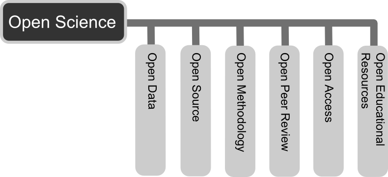
The Open Science movement encourages researchers to share research output beyond the contents of a published academic article (and possibly supplementary information).

FAIR principles

(This image was created by Scriberia for The Turing Way community and is used under a CC-BY licence. The image was obtained from https://zenodo.org/record/3332808)

“FAIR” is the current buzzword for data management. You may be asked about it in, for example, making data management plans for grants:

Findable
- Will anyone else know that your data exists?
- Solutions: put it in a standard repository, or at least a description of the data. Get a digital object identifier (DOI).
Accessible
- Once someone knows that the data exists, can they get it?
- Usually solved by being in a repository, but for non-open data, may require more procedures.
Interoperable
- Is your data in a format that can be used by others, like csv instead of PDF?
- Or better than csv. Example: 5-star open data
Reusable
- Is there a license allowing others to re-use?

Even though this is usually referred to as “open data”, it means considering and making good decisions, even if non-open.

FAIR principles are usually discussed in the context of data, but they apply also for research software.

Note that FAIR principles do not require data/software to be open.

Think about open science in your own situation

Do you share any other research outputs besides published articles and possibly source code?
Is there any particular reason which stops you from sharing research data?

Exercises

Use Xarray to work with NetCDF files

This exercise is derived from Xarray Tutorials, which is distributed under an Apache-2.0 License.

First create an Xarray dataset:

import numpy as np
import xarray as xr

ds1 = xr.Dataset(
    data_vars={
        "a": (["x", "y"], np.random.randn(4, 2)),
        "b": (["z", "x"], np.random.randn(6, 4)),
    },
    coords={
        "x": np.arange(4),
        "y": np.arange(-2, 0),
        "z": np.arange(-3, 3),
    },
)
ds2 = xr.Dataset(
    data_vars={
        "a": (["x", "y"], np.random.randn(7, 3)),
        "b": (["z", "x"], np.random.randn(2, 7)),
    },
    coords={
        "x": np.arange(6, 13),
        "y": np.arange(3),
        "z": np.arange(3, 5),
    },
)

Then write the datasets to disk using to_netcdf() method:

ds1.to_netcdf("ds1.nc")
ds2.to_netcdf("ds2.nc")

You can read an individual file from disk by using open_dataset() method:

ds3 = xr.open_dataset("ds1.nc")

or using the load_dataset() method:

ds4 = xr.load_dataset('ds1.nc')

Tasks:

Explore the hierarchical structure of the ds1 and ds2 datasets in a Jupyter notebook by typing the variable names in a code cell and execute. Click the disk-looking objects on the right to expand the fields.
Explore ds3 and ds4 datasets, and compare them with ds1. What are the differences?

Get a DOI by connecting your repository to Zenodo

Digital object identifiers (DOI) are the backbone of the academic reference and metrics system. In this exercise you will see how to make a GitHub repository citable by archiving it on the Zenodo archiving service. Zenodo is a general-purpose open access repository created by OpenAIRE and CERN.

For this exercise you need to have a GitHub account and at least one public repository that you can use for testing. If you need a new repository, you can fork for example this one (click the “fork” button in the top right corner and fork it to your username).

Sign in to Zenodo using your GitHub account. For this exercise, use the sandbox service: https://sandbox.zenodo.org/login/. This is a test version of the real Zenodo platform.
Go to https://sandbox.zenodo.org/account/settings/github/ and log in with your GitHub account.
Find the repository you wish to publish, and flip the switch to ON.
Go to GitHub and create a release by clicking the Create a new release on the right-hand side (a release is based on a Git tag, but is a higher-level GitHub feature).
Creating a new release will trigger Zenodo into archiving your repository, and a DOI badge will be displayed next to your repository after a minute or two.
You can include the DOI badge in your repository’s README file by clicking the DOI badge and copy the relevant format (Markdown, RST, HTML).

Scientific Data

Types of scientific data

Bit and Byte

Numerical Data

Text Data

Metadata

Data and storage format

Tabular data structure

Gridded data structure

An overview of common data formats

CSV (comma-separated values)

HDF5 (Hierarchical Data Format version 5)

NetCDF4 (Network Common Data Form version 4)

There’s more

Xarray

Sharing data

Pros and cons of sharing data (from Wikipedia)

FAIR principles

Services for sharing and collaborating on research data

Exercises

See also