Background: universal MLIPs

The webinar slides for this page: Webinar slides (PDF).

Objectives

• Define a foundation MLIP and its training data.

• Explain why most materials models miss dispersion.

• Choose and check a model and a GPU engine.

Core concepts for the hands-on parts. Numbered references are at the end; reviews are in Further reading.

Interatomic potentials and MLIPs

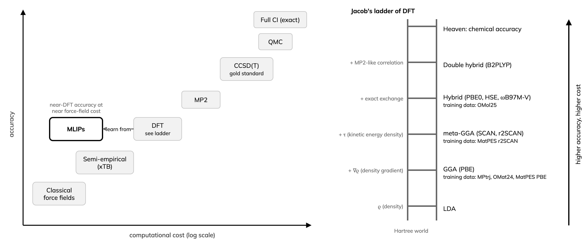
• A potential gives energy from atomic positions; its gradient gives the forces for molecular dynamics (MD) and relaxation.

• Classical force fields: fixed functional form, fast, limited transferability. First-principles (quantum-mechanical) methods such as density functional theory (DFT): accurate, cost grows steeply with system size.

• An MLIP is trained on first-principles (DFT) energies and forces: near-DFT accuracy at near force-field cost. The idea dates from 2007 [1].

• An MLIP inherits the accuracy of the reference method it was trained on (usually PBE DFT), not more: it reuses that rung’s accuracy at a fraction of its cost.

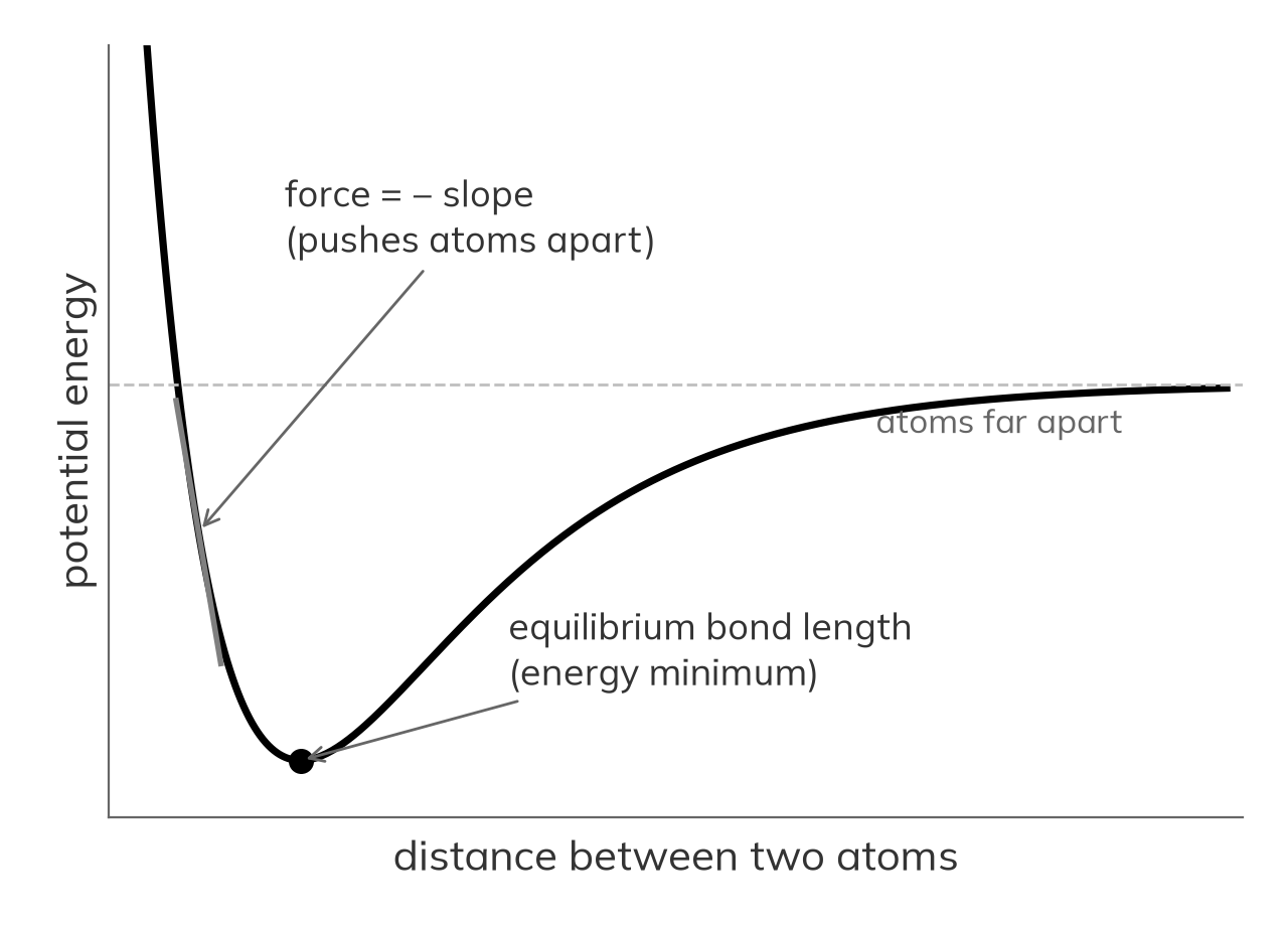
Energy of two atoms versus their distance (illustrative Morse curve).

MLIPs among AI methods for materials

Six families, often confused. They differ in what the model learns or does.

Electronic structure

learns the quantum mechanics itself

• Neural wavefunctions (FermiNet, PauliNet)

• Learned XC functionals (DM21, Skala)

• ML Hamiltonians and tight-binding (DeepH)

Interatomic potentials

learns energies and forces from DFT data

• Universal models (MACE-MP, UMA, Orb, MatterSim, NequIP-OAM)

• Fine-tune a foundation model on your own data

Generative models

proposes new structures on demand

• Diffusion for crystals (CDVAE, MatterGen)

• Language models write crystal files (CrystaLLM)

• Organic crystal prediction (Clari, 2026)

Structure to property

maps a structure straight to a property

• Descriptors (SOAP, matminer)

• Crystal graph networks (CGCNN, ALIGNN)

• Multi-task models (MatterSim-MT, 2026)

LLMs and agents

reads, plans and runs the tools

• Chemistry agents (ChemCrow, Coscientist)

• Simulation agents (MDCrow, El Agente, AtomisticSkills)

• LLM with an MLIP encoder (MatterChat)

Autonomous labs, open data

closes the loop: predict, make, measure

• Self-driving labs (A-Lab, robotic chemist)

• Open data (OMat24, Alexandria, LeMaterial)

• Predicted stable is not always synthesisable [34, 35]

How they connect:

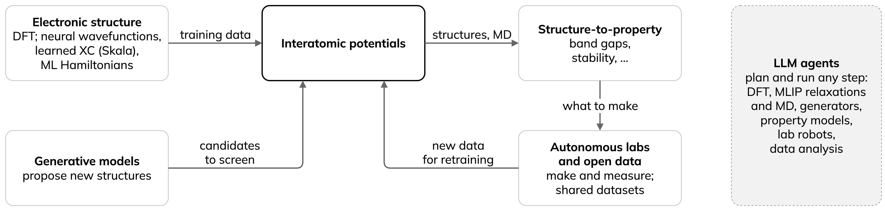
• MLIPs sit in the middle: first-principles data in, structures and dynamics out.

• Generators propose, MLIPs screen, labs make; new data feeds retraining.

• LLM agents can run any step, from one DFT or MLIP calculation to the whole loop.

• This lesson covers interatomic potentials only.

Next door, fast quantum chemistry (outside this lesson’s hands-on scope): the Grimme group’s xTB methods need no training data, cover any element and give electronic information. g-xTB approaches hybrid-DFT quality for elements H to Lr [25]; CREST samples with xTB and an MLIP can refine the result [26]. The two also meet: NN-xTB tunes the xTB Hamiltonian with a network [27], xTB features help ML screen MOF band gaps [28], and dxtb is differentiable xTB in PyTorch [29]. D3 and D4 dispersion add the van der Waals that PBE-trained MLIPs miss; they now run on the GPU in TorchSim and with Orb, and a faster D3 for large cells appeared in 2026.

Use xTB when	Use an MLIP when	Combine them
Chemistry absent from MLIP training data	System within the training distribution	Conformer search with xTB (CREST), energies refined with the MLIP
Unusual elements, charge or spin states	Near-DFT accuracy in that domain	xTB as a cross-check outside the MLIP’s domain
Electronic properties: charges, orbitals, gaps	Large systems, long MD: linear scaling, GPUs	D3/D4 dispersion added to either

From bespoke to foundation models

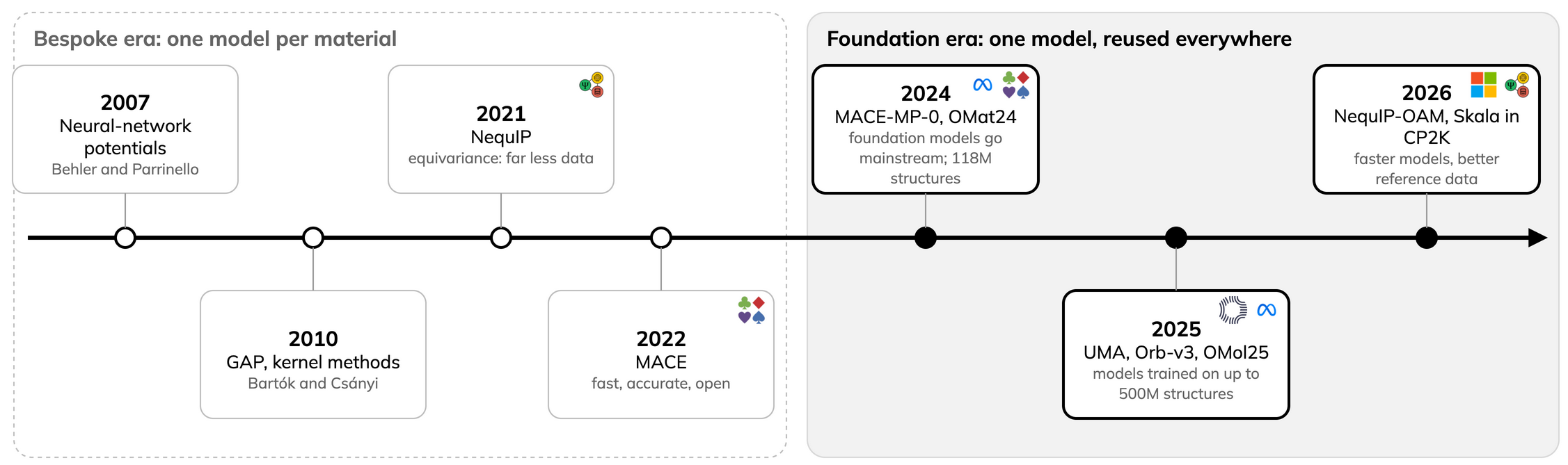
MLIP milestones, from one model per material to one model reused everywhere. Logos identify the developing organisations.

• System-specific MLIP: trained for one material, refitted for the next.

• Equivariant graph networks, NequIP [2] and MACE [3], need far less data.

• Foundation MLIP: pre-trained across the periodic table, reused without retraining. MACE-MP-0 [4] made zero-shot use mainstream in 2024; UMA [7] and Orb-v3 [8] followed in 2025.

• UMA shows the scale: one model trained on about 500 million structures from five datasets. Its mixture of linear experts stores 1.4 billion parameters (UMA-M) and blends them per structure into one model of about 50 million, so inference stays affordable. OMol25 adds hybrid-DFT molecules. Use the current checkpoint (UMA 1.2 small, patch 1.2.1); the original uma-s-1 is archived [7]. A6 One model for materials and molecules: Orb and UMA sets it beside Orb-v3 and OrbMol, on crystals and on molecules with charge and spin.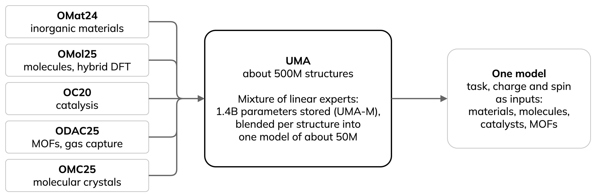

  

• The training level matters: for electrolyte densities, the OMol25-trained UMA reached R² 0.98 against 0.34 and 0.45 for materials-only models [23]; see the molecular row of Choosing an MLIP.

  

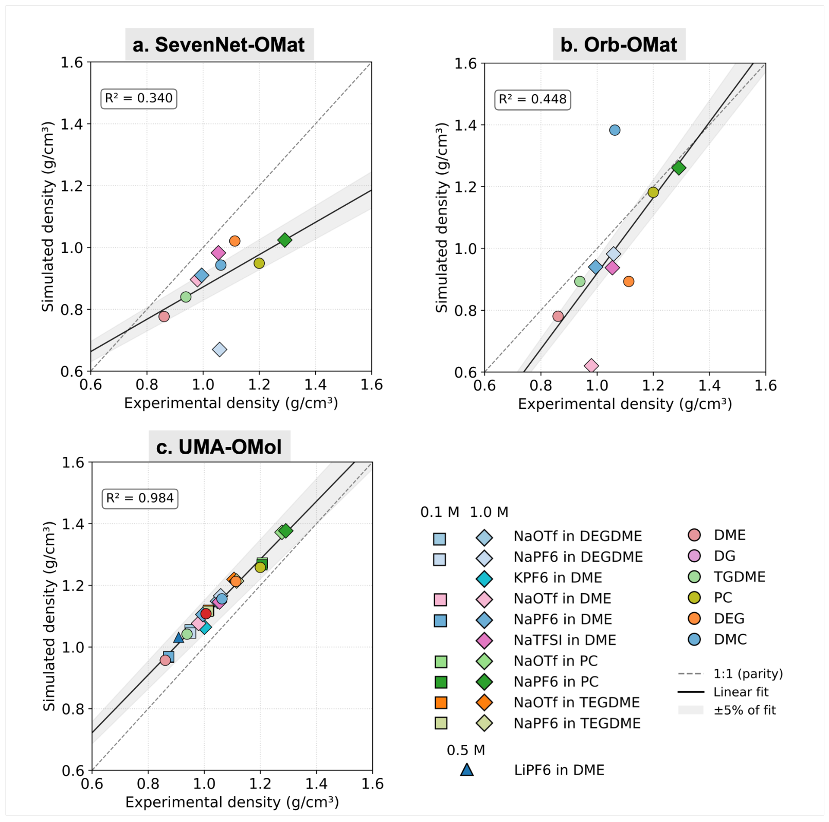
  Kumar et al., arXiv:2603.20183, Fig. 1 (CC BY 4.0, cropped).

• Coverage follows the data: common elements appear in hundreds of thousands of structures, rare ones (noble gases) in a handful (MPtrj counts in [4]). Check your elements and short-range repulsion before screening arbitrary crystals.

  

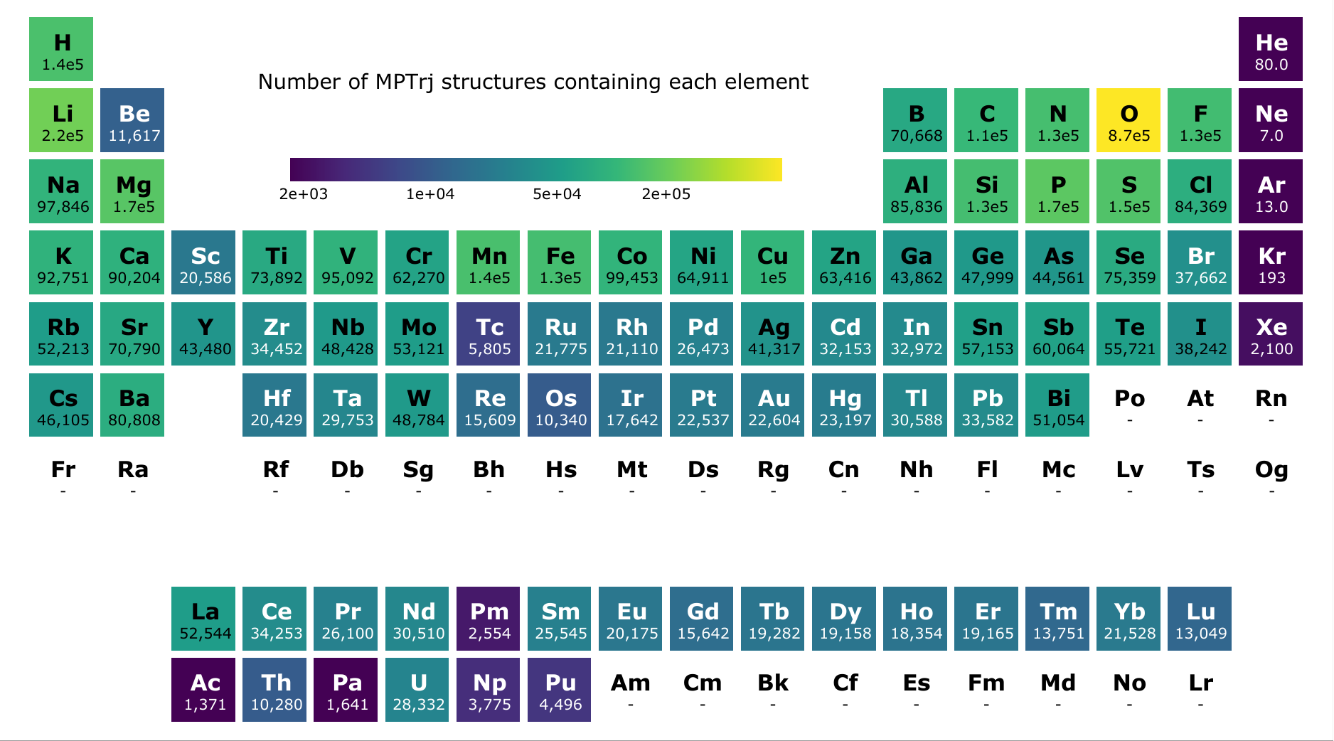
  Number of MPtrj structures containing each element. Matbench Discovery (MIT).

Training data grew over a hundredfold in a few years:

Dataset	Scale	Reference level
MPtrj [5]	about 1.58 million configurations, about 146,000 Materials Project compounds, 89 elements	PBE(+U)
MatterSim	about 17 million configurations (active learning)	PBE(+U)
GNoME	about 89 million structures (not public)	PBE(+U)
OMat24 [6]	about 118 million inorganic structures	PBE+U
OMol25 [9]	more than 100 million calculations, about 83 million molecular systems, 83 elements	ωB97M-V/def2-TZVPD
UMA training [7]	about 500 million unique 3D structures	mixed

Model families (figures as published; the field moves fast):

Model family	From	Architecture	Params	Training data
CHGNet, 2023 [5] (code)	UC Berkeley	GNN with magnetic moments	0.4M	MPtrj
MACE-MP-0, 2024 [4] (code)	Cambridge and others	equivariant message passing (ACE)	4.7M	MPtrj; newer multi-head models add more
SevenNet-0, now Omni [Omni] (code)	SNU	NequIP-style equivariant GNN	0.8M, now 55M	MPtrj, now 243M structures
Orb-v3 [8] (code)	Orbital Materials	non-equivariant graph network	26M	OMat24, or MPtrj plus Alexandria
eqV2, eSEN, UMA [6] [eSEN] [7] (code)	Meta FAIR	equivariant transformer, then eSEN with a mixture of linear experts	31M to 153M; UMA up to 1.4B (50M active)	OMat24, then about 500M
DPA-3, now DPA-4 and DPA4C [18] (code)	AISI Beijing, DP Technology	line-graph GNN, now SO(3)-equivariant	0.03M to 25M	OpenLAM (163M)
NequIP and Allegro OAM, 2026 [12] (NequIP, Allegro)	Harvard, Cambridge	E(3)-equivariant; Allegro strictly local	0.6M to 32M	OAM
PET-OAM, 2026 [PET] (code)	EPFL	transformer, symmetry not enforced	26M to 730M	OAM
GRACE [GRACE] (code)	ICAMS, Bochum	graph atomic cluster expansion	3.4M to 42M	MPtrj; OAM

OAM = OMat24 + sAlex + MPtrj. MatterSim [24] and other fast models are compared in the fast-models table below.

Materials models learn PBE, which misses dispersion, so A2 Orb-v3, MatGL and dispersion adds D3. OMol25 models use a different reference level.

How the models are built

First papers and code: Behler and Parrinello 2007 (code), GAP 2010 (code), SNAP 2015 (code), MTP 2016 (code), ANI-1 2017 (code), ANI-1ccx, CCSD(T) data, SchNet (code), DeePMD 2018 (code), ACE 2019 (code), NequIP (code), MACE (code), M3GNet (code), CHGNet (code), MACE-MP-0 (code), UMA (code), Orb-v3 2025 (code), NequIP-OAM 2026 (code), DPA4C 2026 (code), Skala, learned DFT (code).

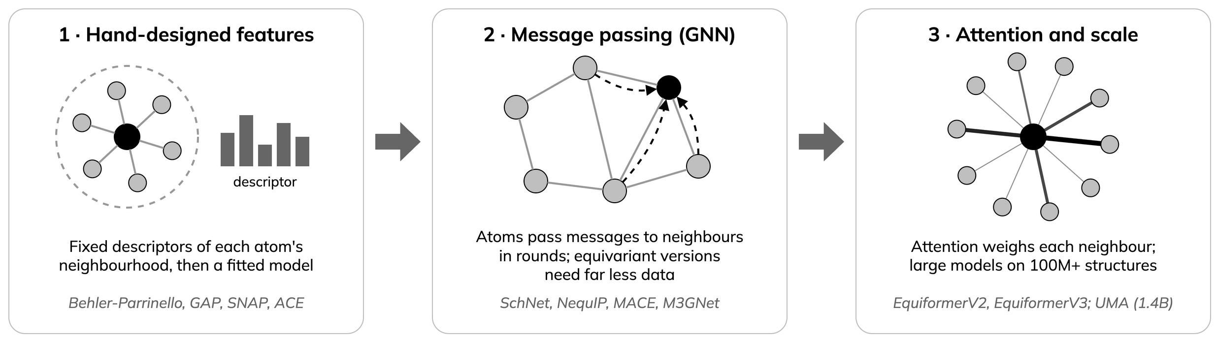
• Message passing: in a graph neural network (GNN), atoms exchange information with neighbours over several rounds; features are learnt, not hand-designed.

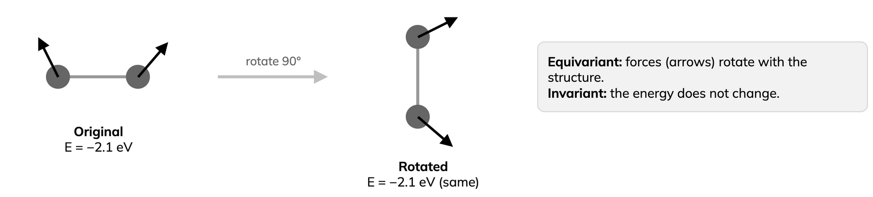
• Equivariant: rotate the structure and the predicted forces rotate with it, while the energy is unchanged. NequIP needs up to about 1000 times less data [2].

• Attention (EquiformerV2 [paper], EquiformerV3 [paper]) weighs each neighbour; models such as UMA (1.4B parameters) train on 100M+ structures. By 2026, simpler designs compete closely [Orb-v3]: data and scale matter more than architecture.

Pre-train, then fine-tune

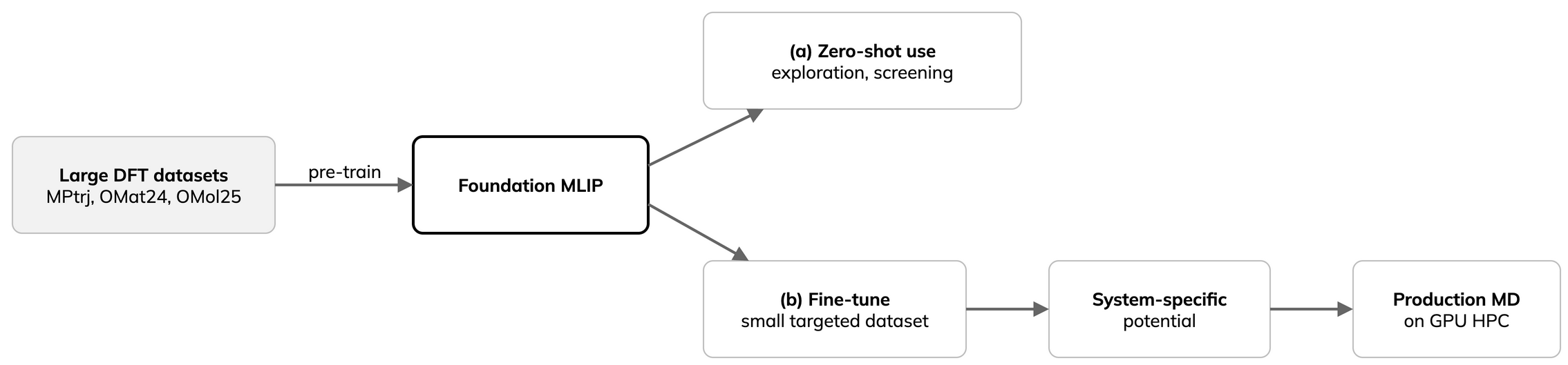
Recipe [10]:

1 · Start zero-shot

Use the foundation model directly; often good enough for screening.

2 · Fine-tune

Add a small, targeted dataset when you need numbers for one system.

3 · Select data

Uncertainty-aware sampling adds what the model is least sure about.

4 · Validate

Test the property that matters, not just the energy.

Catastrophic forgetting: a network trained further on new data can lose accuracy on what it learnt before [EWC]. Fine-tuned universal MLIPs show it too, and forgetting-aware fine-tuning limits it [16]. Keep the original model for general use.

Where zero-shot models fall short: used as-is, foundation models get structures right but can be far off on mechanical and disordered systems; fine-tuning usually needs less data than training from scratch and closes most of the gap.

• Fine-tuned models have lower energy errors at every data fraction, with the biggest gain at 10%; force errors converge with from-scratch training as data grows [10].

  

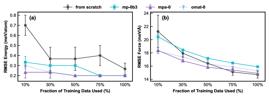
  Learning curves, fine-tune against from scratch, Liu et al., J. Appl. Phys. 139, 041101 (2026) (CC0).

System, model	Property	Zero-shot	Fine-tuned
Mo, MACE-MP-0b3 [10]	$C_{11}$ elastic constant, error	45.9%	2.6%
Mo, MACE-MP-0b3 [10]	stacking-fault energy	far too low	close to DFT
Si, MACE-MP-0b [Si]	elastic constants, error	19 to 53%	0.6 to 5.2%
High-entropy alloy, MACE-MP-0 [HEA]	energy error, meV/atom	59 to 64	13.8 (from scratch: 16.4 MACE, 24.1 ACE)
41 models on a-C and a-SiO2 [17]	energy error	above 100% for some (a-C)	more than 5x lower from 4 structures (a-SiO2)

• Elastic constant: how stiff a material is. Stacking-fault energy: the cost of sliding atomic layers, which sets how metals deform.

  

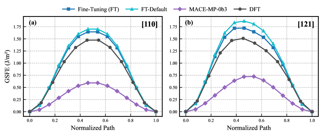
  Mo stacking-fault energy: MACE-MP-0b3 (purple), DFT (black), fine-tuned (blue). Liu et al., J. Appl. Phys. 139, 041101 (2026) (CC0).

• Our own run, A4 Train and fine-tune a potential: TensorNet (MatPES-PBE) fine-tuned to r2SCAN on 84 Li structures reaches 60 meV/atom energy and 128 meV/Å force error, against 513 and 427 from scratch (one run, one MI250X GCD).

GPU engines

CPU-era simulation tools

• Built to run one system at a time

• GPU speed-ups first targeted classical force fields

• Excellent for cheap, simple functional forms

GPU-era foundation MLIPs

• Neural networks with millions of parameters

• Want batched inference: many structures per GPU call

• One structure at a time leaves the GPU mostly idle

• TorchSim (PyTorch; paper, code, docs), kUPS (JAX; code, blog) and NVIDIA ALCHEMI Toolkit (PyTorch and Warp; code, docs, blog) batch many systems into one GPU call. Part A uses TorchSim; Part B uses ALCHEMI Toolkit. All three are open source.

  Engine	Stack	Idea	Licence
  TorchSim	PyTorch	batched MD, relaxation and Monte Carlo; drives MACE, FairChem/UMA, SevenNet, ORB, MatterSim	MIT (Radical AI)
  kUPS	JAX	differentiable MD, Monte Carlo and optimisation primitives; runs MACE and UMA	Apache-2.0 (CuspAI)
  ALCHEMI Toolkit	PyTorch and Warp	vendor toolkit; batched and multi-GPU MD and relaxation with MACE, AIMNet2, UMA, MatGL TensorNet	Apache-2.0 (NVIDIA, v0.2.0)

• What batching changes:

  One system per call

  Classical tools and ASE: one structure at a time, hardware mostly idle.

  Many systems per call

  GPU-native engines fill the card with a batch.

  Up to about 100x

  TorchSim against ASE on one H100: total throughput, not per system [paper].

  5 to 7x

  Our A100 runs, 64 to 128 relaxations (A1 Batched relaxation for screening).

  

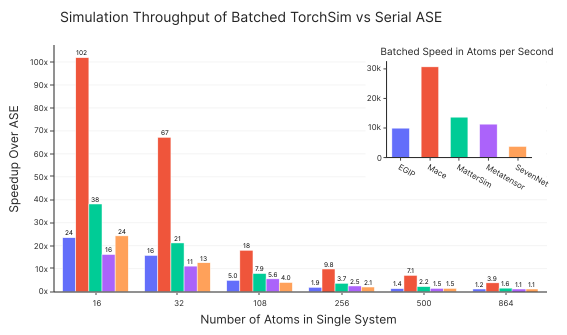
  Throughput vs ASE (single H100, batched). TorchSim (MIT).

  This makes relaxing and screening large candidate sets practical.

• ALCHEMI also supplies common GPU building blocks (neighbour lists, D3 dispersion, Ewald sums; Toolkit-Ops, docs, blog) used by UMA, Orb, PET and TorchSim. These run on NVIDIA GPUs only; the D3 on A2 Orb-v3, MatGL and dispersion also runs on a CPU.

Engines are built from swappable blocks: the same potential, integrator and thermostat give NVE, NVT or NPT. After the kUPS design (CuspAI, 2026).

• Leonardo (NVIDIA A100; Booster nodes with four GPUs each): CUDA-native, so TorchSim, cuEquivariance and ALCHEMI run directly. Our batched relaxation gave 5 to 7x over serial (A1 Batched relaxation for screening).

• LUMI (AMD MI250X; LUMI-G nodes with four MI250X, each two GCDs): ROCm PyTorch runs MACE, NequIP and MatGL (float64); CUDA-only kernels do not. Our MACE, MatGL, fine-tuning and NEB runs used one GCD (A1 Batched relaxation for screening, A3 MatGL: relaxation, MD, lattice benchmark and training to A5 NEB: migration barriers with MLIPs). TorchSim added AMD/ROCm support in v0.4.2, verified on consumer cards. Docs: docs.lumi-supercomputer.eu.

• Arrhenius (NVIDIA GH200, Linköping, inaugurated September 2026): 382 nodes with four Grace Hopper superchips each; CUDA-native [NAISS]. Part B ran here: eight 64-atom MACE silicon trajectories on one GH200 took 18.7 s as one ALCHEMI batch versus 88 to 100 s as eight LAMMPS processes (B7 Read a completed shared-GPU benchmark); one LAMMPS system on four GPUs ran 2.4 times faster than on one (B8 One silicon simulation on more than one GPU). Setup: Arrhenius setup.

• ENCCS and Sweden AI Factory help with access and the software stack; Sweden AI Factory’s own AI-optimised system in Linköping follows in 2026/2027.

• NequIP and Allegro foundation models run LAMMPS ML-IAP/Kokkos MD on both: up to 102.5 million atoms on 256 GPUs, about 44 000 atoms per A100 and 22 000 per MI250X GCD. NequIP-OAM-XL matches eSEN-30M-OAM on Matbench Discovery at about ten times the speed [12].

• DPA4C (DeePMD-kit v3.2.0) approaches MACE-OMat accuracy at about 100 times the throughput; 2.048 billion atoms on 1024 V100 GPUs [18]. Checkpoints are CC-BY-NC.

• LUMI tip: with the CSC PyTorch module (torch 2.7.1+rocm6.2.4), torch.det and prod fail in float32 on the MI250X but work in float64, so MatGL runs in float64 there (A3 MatGL: relaxation, MD, lattice benchmark and training, A4 Train and fine-tune a potential).

• Measured multi-GPU MACE scaling: B8 One silicon simulation on more than one GPU.

Note

Pin software versions and re-check results after upgrades. Bugs that silently gave wrong results were fixed between July and September 2026 in cuEquivariance v0.12.0 (fused tensor-product reduction), NequIP v0.19.0 (wrong forces and stress in TorchSim) and TorchSim v0.6.1 (D3, Ewald, PME and DSF stress sign) [19].

Choosing and trusting a model

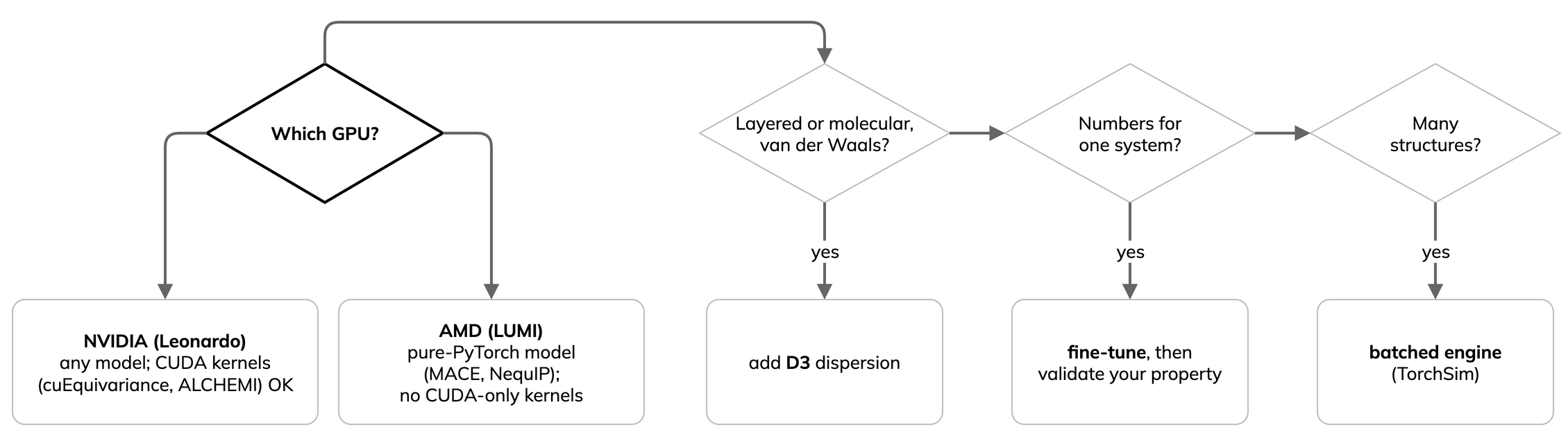
• Choose by task and hardware, not by the top leaderboard row.

• Validate the property you study; compare several models.

• Rules of thumb, a check protocol and the evidence behind them: Choosing an MLIP.

Fast universal models (Matbench Discovery data, accessed 29 September 2026 [13]):

Model	Params	F1 ↑	κSRME ↓	Licence	Use case
Orb-v3 [8]	26M	0.905	0.21	Apache-2.0	fast; D3 variant for van der Waals
SevenNet-Omni [paper]	55M	0.906	0.19	MIT	D3 built in; LAMMPS and TorchSim
NequIP-OAM-XL [12]	32M	0.906	0.13	MIT / CC-BY	also runs on AMD GPUs (LUMI)
MatRIS-10M-OAM [paper]	10M	0.921	0.22	BSD-3	best accuracy for its size
MatterSim v1 5M [24]	4.5M	0.862	0.57	MIT	small and fast
Nequix [paper]	0.7M	0.751	0.45	MIT / CC-BY	cheapest to run and train
eSEN-30M-OAM [paper]	30M	0.925	0.17	MIT / gated	very accurate; UMA family
EquiformerV3-OAM [paper]	30M	0.931	0.12	MIT	accuracy leader, slower

• Matbench Discovery is the main public leaderboard for crystal stability: does a predicted crystal hold together or decompose? F1 (0 to 1, higher is better): stable-crystal classification on Matbench Discovery [13]. κSRME (lower is better): thermal-conductivity error.

• F1 combines two questions. Precision: of the crystals the model calls stable, what share are stable? Recall: of the truly stable crystals, what share does it find? $F_1 = 2PR/(P+R)$, so a model must do well on both.

• Models are ranked by CPS, a combined score: 50% F1, 40% κSRME and 10% structure error (RMSD). The compliant tier trains on MPtrj only, for a fair comparison. Since July 2026 there is also an MD task.

  

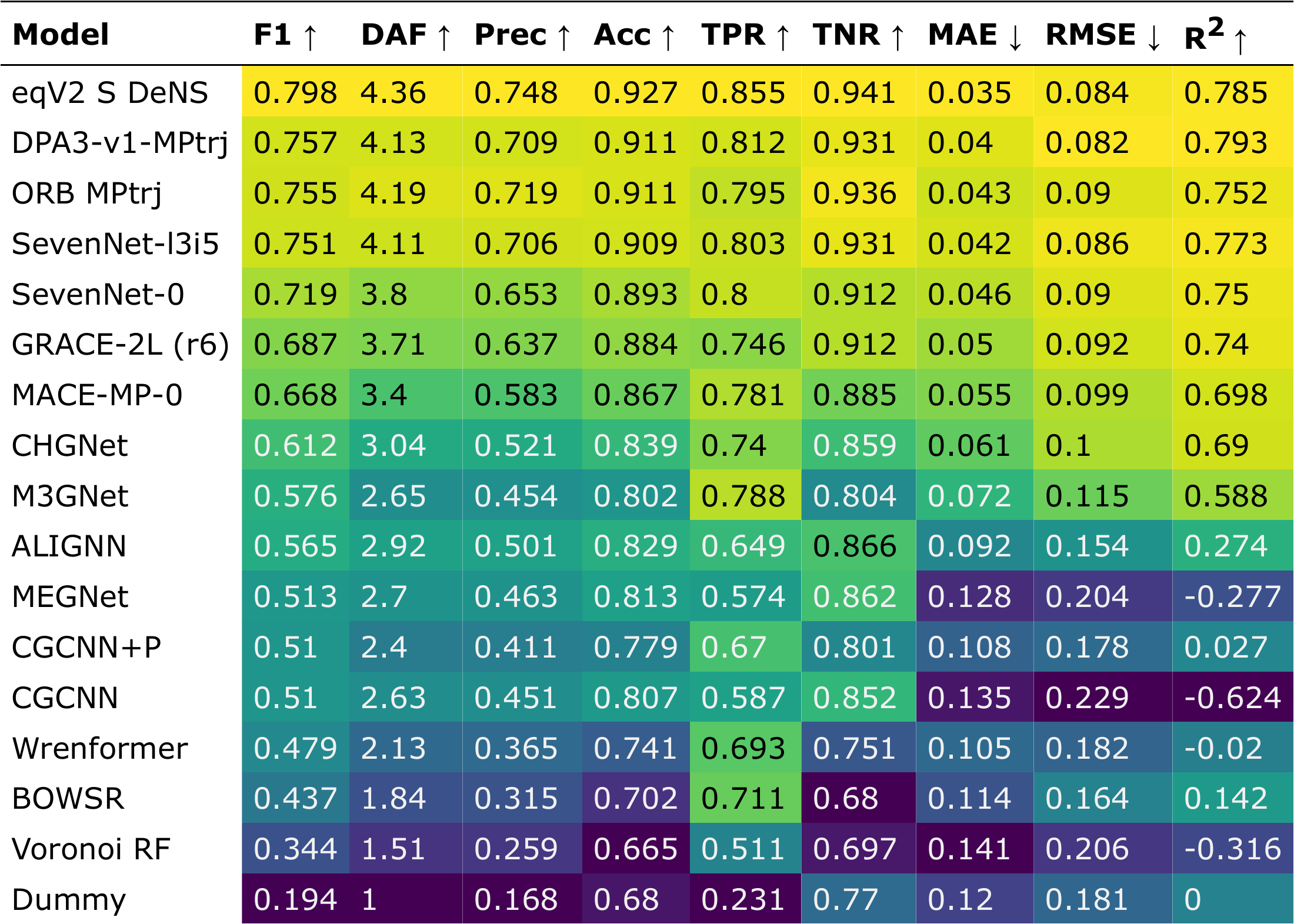
  Compliant (MPtrj-only) models, 2025 paper snapshot; best today is F1 ≈ 0.86 (EquiformerV3). Matbench Discovery [13]. PBE references; not a Materials Project endorsement.

• MatGL 4.0.3 (BSD-3) models (TensorNet, CHGNet, M3GNet and QET trained on MatPES; used in A2 to A4) are not on the leaderboard. MatGL has no TorchSim interface, so it runs through ASE.

• The compliant tier fixes the training data to MPtrj, so architectures are compared fairly; the best compliant F1 today is about 0.86 (EquiformerV3).

• The leaderboard is a moving target:

  Year	Model	Training data	F1
  2023	CHGNet	MPtrj	0.61
  2024	MACE-MP-0	MPtrj	0.67
  2024	eqV2	OMat24	0.92
  2025	Orb-v3	OMat24	0.91
  2026	EquiformerV3	OMat24 and more	0.93

  In three years F1 rose from about 0.6 to 0.93, mainly from more and broader training data. With training fixed to MPtrj (compliant tier), the best went from 0.82 (2024) to about 0.86 today. The top models are now within a few hundredths, so choose by your task, speed and licence.

• Most GPU speed-ups are NVIDIA-only (Leonardo, Arrhenius). On AMD (LUMI), choose a pure-PyTorch model such as NequIP or MACE.

• A low force error is not enough: check MD stability, speed, memory and your property [Forces are not enough; code].

• Finite-temperature MD of 15 foundation MLIPs, tier medians [20]:

  Tier (training data)	Force RMSE, eV/Å	Pressure MAE, GPa
  1 (MPtrj)	0.166	0.82
  2 (+ Alexandria)	0.106	1.04
  3 (OMat24-based)	0.063	0.82
  4 (multi-dataset)	0.054	3.40

  The tier with the lowest force error has the worst pressure error, driven by the UMA models on one alloy (an unrelaxed experimental cell). It is now the Matbench Discovery MD task.

  

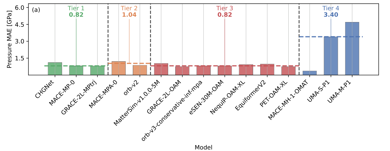
  Gawkowski et al., arXiv:2607.03433, Fig. 4(a) (CC BY-SA 4.0, cropped).

• Molecules, 15 pretrained models, MD of a 2,661-atom water box on one H100 [15]: accuracy tracks model size and data, but slower is not always more accurate.

  Model	Energy MAE, kcal/mol	MD steps/s
  UMA-m-1.1	0.53	0.16
  UMA-s-1.1	0.61	3.65
  MACE-OFF23 (L)	1.73	1.43
  AIMNet2	2.55	33.7

• Beyond one score: MLIP Arena (leaderboard) [14] tests physics in four groups: asymptotic behaviour (diatomic curves, energy conservation), stability and reactivity (heating, compression, combustion), distribution shifts (gas adsorption, vacancy migration) and thermodynamics (equation of state, phase transitions). In its heating test, 120 NVT runs from 300 to 3000 K in 10 ps on one A100, the share of valid runs ranges from about 97% (ORBv2) to about 44% (M3GNet).

  

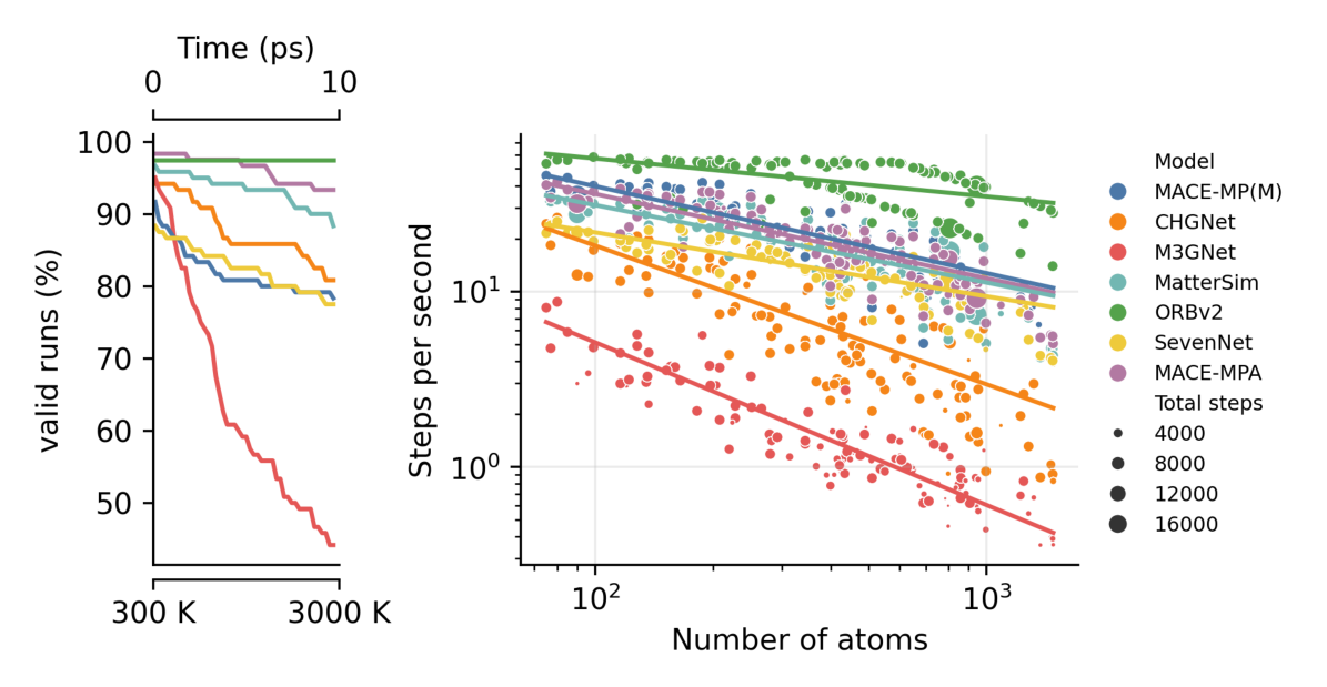
  Chiang et al., arXiv:2509.20630, Fig. 3(a) (CC BY 4.0, cropped).

• For molecules, mlipbenchmarks [15] compares accuracy, MD speed and GPU memory for 15 models; all ran stable MD, so accuracy against speed decides.

• Ensemble: run several models; disagreement flags low confidence.

• Check speed and GPU memory at your system size.

• PBE-trained models miss dispersion. Grimme’s D3 correction adds it on the GPU in TorchSim and orb-models (used on A2 Orb-v3, MatGL and dispersion).

Barriers and NEB

• Diffusion and reactions are set by the barrier E_a at a saddle point, and the rate depends on it exponentially: at 298 K, 60 meV is about a factor of ten in diffusivity [38].

• The climbing-image nudged elastic band (CI-NEB) finds the saddle with a chain of images between two minima [36]. Each image needs one force call per step, so an MLIP runs it in seconds on a GPU.

  

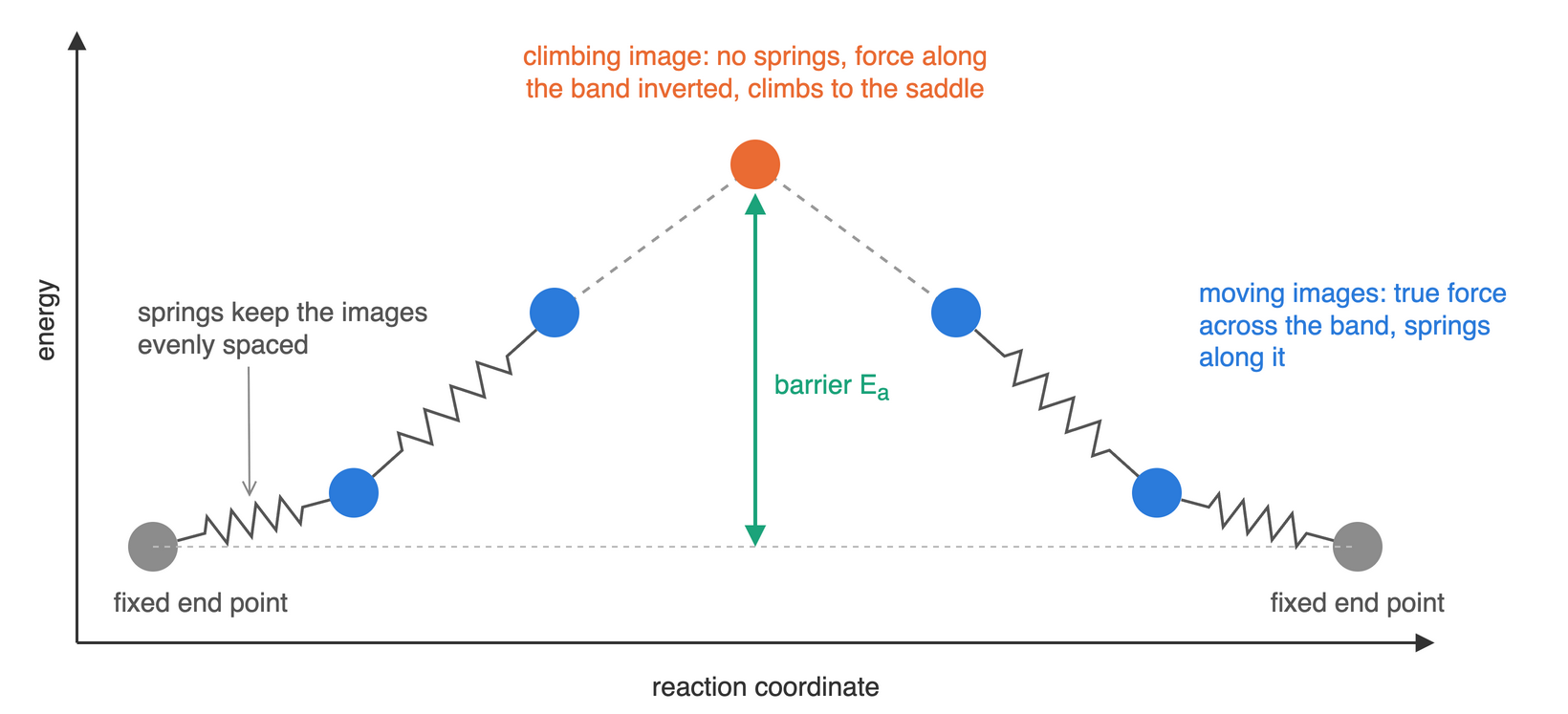
• NEB relaxes 5 to 9 images together. With DFT that is hundreds to thousands of DFT calls per path; with an MLIP each force call takes milliseconds, so thousands of paths become practical. CatTSunami ran a CO hydrogenation network on Rh(111), 19,000 NEBs, in 12 GPU days, against an estimated 52 GPU years with DFT [39].

• Universal MLIPs soften the energy surface far from equilibrium and tend to underestimate barriers: MAE 0.34 (MACE), 0.39 (CHGNet) and 0.49 eV (M3GNet) for 470 Mg²⁺ paths [37]; CHGNet and M3GNet underestimate 73 % and 78 % of 574 paths [38].

• For those 574 battery paths: MAE 0.31 (MACE-MP-0) to 0.35 eV (M3GNet), and 0.20 to 0.26 eV without each model’s outliers above 1 eV; good or bad conductor at 0.5 eV right 74 % (M3GNet) to 85 % (Orb-v3) of the time; MLIP paths were a better DFT starting guess in about two thirds of cases. DFT-NEB itself carries about 0.06 eV [38].

  

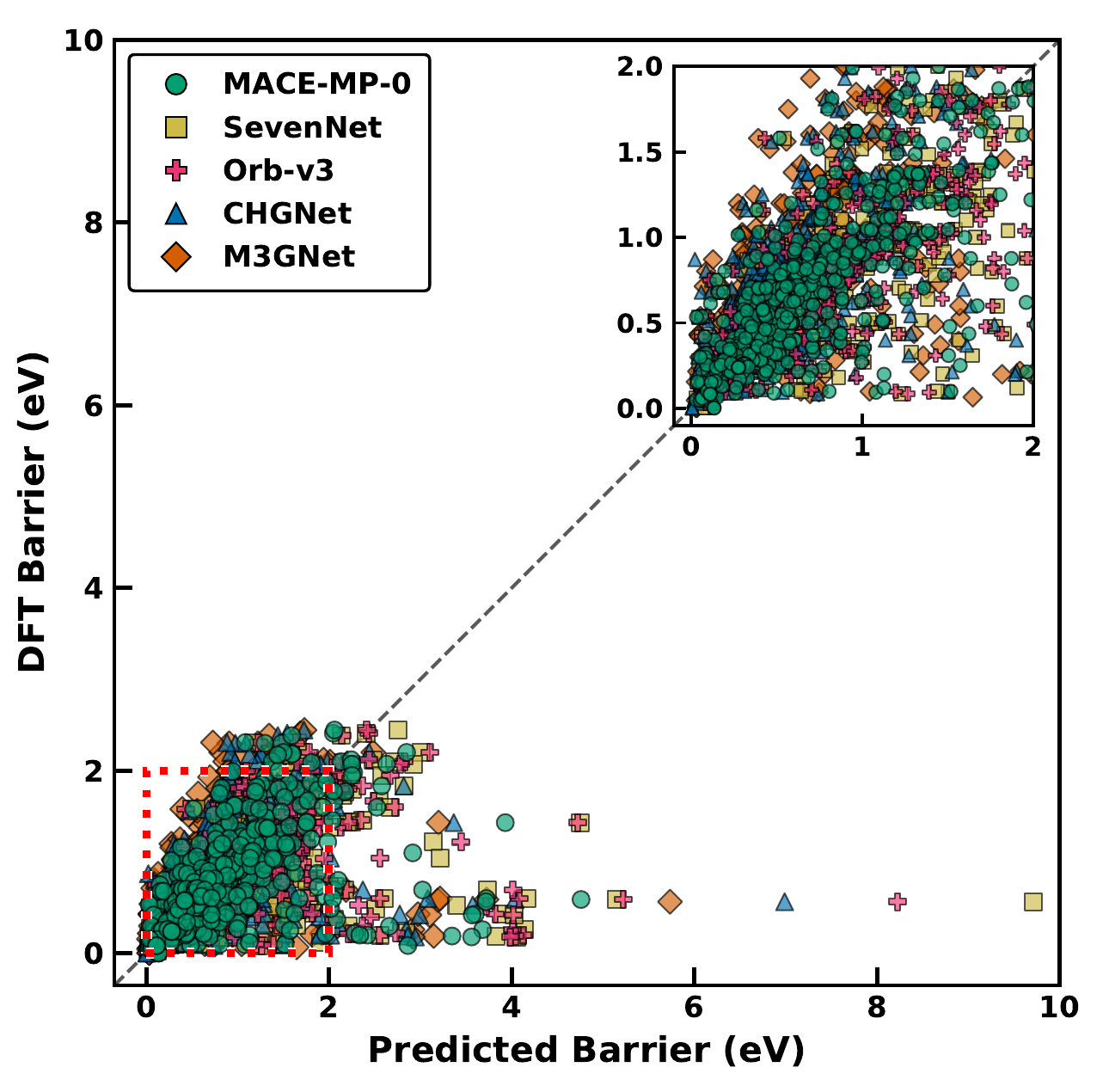
  MLIP vs DFT-NEB barriers, 574 paths. Bheemaguli, Xiao & Sai Gautam, Fig. 2 (CC BY 4.0, cropped).

• Newer models do better (about 0.05 to 0.17 eV on 154 paths) [40]. For 932 surface reactions, MLIP-NEB followed by a few DFT checks put 88 % of barriers within 0.1 eV of DFT at a 28× speed-up [39].

• Pattern: the MLIP finds the path, DFT confirms the saddle. CatTSunami: all-MLIP 2200× faster with 70 % success; adding 2 DFT relaxations and 1 single point gives 88 % at 28× [39]. Molecules: MACE-OMol25 path, then DFT, 96.6 % success with 3.8 DFT gradients per reaction, 94 to 96 % fewer than DFT alone [paper]. Fine-tuning on even one structure removes much of the softening bias [37].

• Use MLIP-NEB to screen and to start DFT, then refine the saddle. Worked example with LiFePO4 on LUMI: A5 NEB: migration barriers with MLIPs.

  

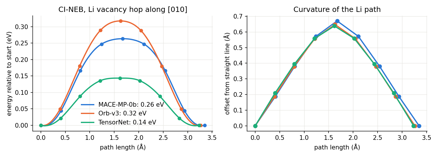
  LUMI run, one MI250X GCD, float64 (A5 NEB: migration barriers with MLIPs).

  MACE-MP-0b 0.26 eV and Orb-v3 0.32 eV fall within 0.05 eV of DFT (GGA 0.27, GGA+U 0.29 eV); TensorNet gives 0.14 eV, as softening predicts. All three find the curved [010] path, 0.64 to 0.67 Å off the straight line. The models cannot place the Fe³⁺ hole, which moves the DFT barrier by almost 0.2 eV.

Outlook

• Long-range physics [30]:

  The gap

  Standard MLIPs see only neighbours within a cutoff, so they miss long-range electrostatics: ions, interfaces, polar materials.

  The idea

  Learn hidden (latent) charges from energies and forces alone, then add the long-range part with an Ewald sum; no charge training data needed.

  What it unlocks

  Born effective charges and polarisation, infrared spectra under a field, ferroelectrics such as PbTiO3, ionic conduction in superionic water.

  

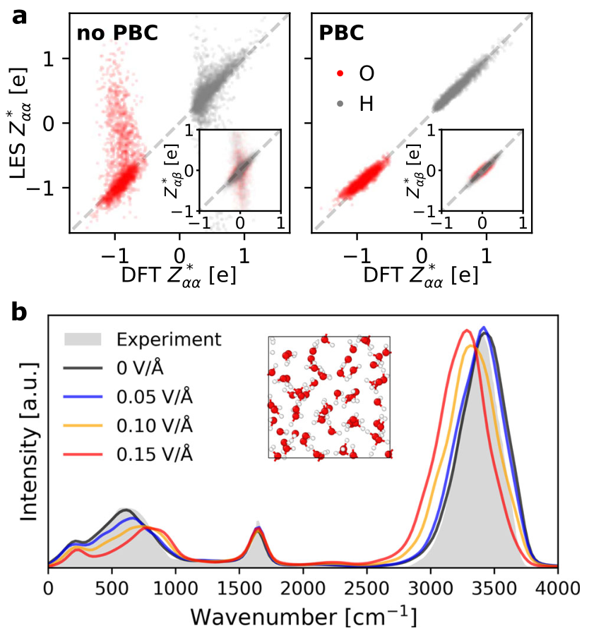
  Zhong, Kim, King and Cheng, npj Comput. Mater. 11, 384 (2025), Fig. 1 (CC BY 4.0, cropped).

• ML inside DFT: DFT is exact except for the exchange-correlation (XC) functional, which must be approximated (the rungs of Jacob’s ladder). Machine learning can learn that term from accurate data:

  Year	Milestone	What it did
  2012	First ML functional	kinetic energy learnt from examples; 1D model systems
  2017	ML density maps	density learnt from the potential, skipping Kohn-Sham steps
  2020	NeuralXC (code)	neural correction on top of a standard XC functional
  2021	DM21, DeepMind [31] (code)	trained with fractional charge and spin; fixes delocalisation error
  2025	Skala, Microsoft [32] (code)	deep-learned XC at meta-GGA cost; beats hybrids on GMTKN55 (2.8 kcal/mol)
  2026	Skala in CP2K (molecular, condensed phase)	molecules (Aug), then condensed phase (Sept): usable for materials

  Skala today: open code (microsoft/skala) with PySCF, GPU4PySCF and ASE interfaces, and now in CP2K for molecular and condensed-phase calculations. Why it matters here: better, cheaper reference data for the next generation of MLIPs; the two directions reinforce each other.

• Generative models propose, MLIPs screen. A diffusion model turns a crystal into noise step by step and learns to run it backwards:

  

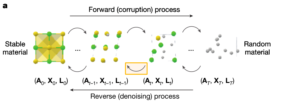
  Zeni et al., Nature 2025, Fig. 1a (CC BY 4.0, cropped).

  MatterGen

  paper, code. Can be steered towards a target chemistry, symmetry or property; more than twice as likely as earlier generators to give stable, unique and new crystals. One candidate was made in the lab; a 2026 study argues it was already known (Mater. Horiz.).

  LeMat-GenBench

  paper, code, leaderboard. Scores 12 generators with an MLIP ensemble (MACE-MP, UMA, Orb); more stable output tends to mean less novel output, and no model wins everywhere. Synthesis and experimental checks remain the real bottleneck.

• Early agentic workflows: agents turn a plain-language goal into simulation steps (plan, call a tool, read the result, repeat).

  

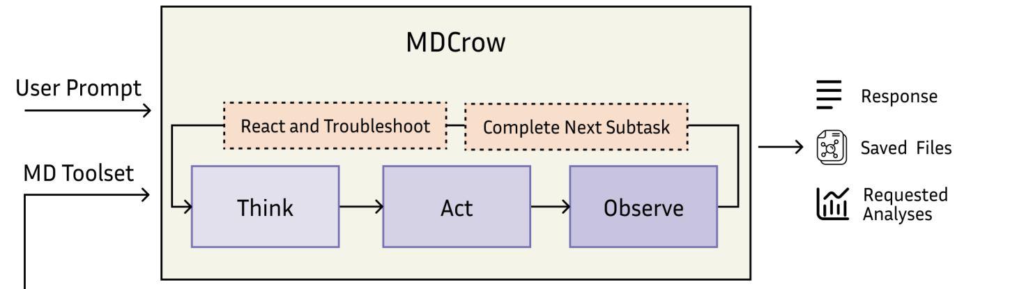
  Campbell et al., arXiv:2502.09565, Fig. 1A (CC BY 4.0, cropped).

  Example	What it does	Result
  MDCrow (code)	MD through OpenMM, 40+ tools	25 tasks: 72% correct (gpt-4o) vs 28% for a bare LLM
  El Agente Q	xTB and ORCA, jobs via SLURM	6 exercises, about 88% average success
  NVIDIA test, Aug 2026	a coding agent wrote 45 batched GPU MACE pipelines	none questioned an ill-posed task; an unstated thermostat damped Li diffusion 3 to 5 times

  Agents can already run the codes, but they do not yet question the physics: expert judgement stays in the loop.

• In every case, validate the property you care about.

“A poorly posed initial question results in AI scientific slop, an unfortunate side effect that is now becoming far too common.” Shyue Ping Ong, September 2026 [22]

Getting started

• Models and code: MACE, SevenNet, Orb, MatterSim, FairChem/UMA, MatGL, DeePMD-kit. Engines: TorchSim, kUPS, ALCHEMI Toolkit.

• Datasets: MPtrj (1.6M configurations, the classic start), OMat24 and OMol25 (100M+ each, materials and molecules), Alexandria (large open DFT database of crystals).

• Benchmarks: Matbench Discovery (stability, κSRME, MD task), MLIP Arena (physical tasks, stability), mlipbenchmarks (molecules, speed, memory).

• Help from ENCCS and Sweden AI Factory: lessons at enccs.github.io/lessons, workshops and events at enccs.se/events; access to LUMI, Leonardo and Arrhenius; compute and AI expertise at swedenaifactory.se; contact training@enccs.se.

Keypoints

• MLIPs learn DFT energies and forces at near force-field cost.

• Use foundation models zero-shot; fine-tune for quantitative accuracy.

• PBE-trained models miss dispersion without D3.

• Batched GPU engines run many systems in one call; choose a model by task and validate the property you study.

• One error number is not enough; pin package versions.

References

1. J. Behler, M. Parrinello, Phys. Rev. Lett. 98, 146401 (2007). doi:10.1103/PhysRevLett.98.146401

2. S. Batzner et al., Nat. Commun. 13, 2453 (2022). doi:10.1038/s41467-022-29939-5

3. I. Batatia et al., MACE. arXiv:2206.07697

4. I. Batatia et al., A foundation model for atomistic materials chemistry. arXiv:2401.00096

5. B. Deng et al., CHGNet and MPtrj, Nat. Mach. Intell. 5, 1031 (2023). doi:10.1038/s42256-023-00716-3

6. L. Barroso-Luque et al., OMat24, Nat. Comput. Sci. 6, 642 (2026). doi:10.1038/s43588-026-00996-w; arXiv:2410.12771

7. B. M. Wood et al., UMA. arXiv:2506.23971

8. B. Rhodes et al., Orb-v3. arXiv:2504.06231

9. D. S. Levine et al., OMol25. arXiv:2505.08762

10. X. Liu et al., J. Appl. Phys. 139, 041101 (2026). doi:10.1063/5.0299305; companion study arXiv:2506.07401

11. TorchSim, kUPS, ALCHEMI Toolkit

12. S. R. Kavanagh et al., NequIP and Allegro foundation models. arXiv:2607.28461

13. J. Riebesell et al., Matbench Discovery, Nat. Mach. Intell. 7, 836 (2025). doi:10.1038/s42256-025-01055-1; leaderboard

14. Chiang et al., MLIP Arena, NeurIPS 2025 Datasets and Benchmarks. arXiv:2509.20630

15. Eastman, Pretti and Markland, mlipbenchmarks, J. Chem. Theory Comput. 22, 6108 (2026). doi:10.1021/acs.jctc.6c00130

16. Kim et al., forgetting-aware fine-tuning of universal MLIPs, npj Comput. Mater. 12, 26 (2026). doi:10.1038/s41524-025-01895-w

17. Fragapane and Deringer, AM26 amorphous-materials benchmark. arXiv:2607.11384

18. DPA4 and DPA4C, DeePMD-kit v3.2.0. arXiv:2608.19041

19. Release notes: cuEquivariance v0.12.0, NequIP v0.19.0, TorchSim v0.6.1

20. Dyna-Mat, foundation MLIPs in finite-temperature MD. arXiv:2607.03433

21. NVIDIA, How AI coding agents can unlock materials simulation with NVIDIA ALCHEMI Toolkit (2026). blog

22. S. P. Ong, The Non-AI-pocalypse in Materials Science (2026). post

23. Kumar et al., electrolyte solvation structure from an OMol25-trained potential. arXiv:2603.20183

24. H. Yang et al., MatterSim. arXiv:2405.04967

25. Froitzheim, Müller, Hansen and Grimme, g-xTB, ChemRxiv (2025). doi:10.26434/chemrxiv-2025-bjxvt

26. Pracht et al., CREST, J. Chem. Phys. 160, 114110 (2024). doi:10.1063/5.0197592

27. Xia, Thie, Soon and Barca, NN-xTB, Nat. Commun. 17, 7302 (2026). doi:10.1038/s41467-026-73184-z

28. Jose and Walsh, J. Chem. Theory Comput. 22, 8531 (2026). doi:10.1021/acs.jctc.6c00979

29. Friede, Hölzer, Ehlert and Grimme, dxtb, J. Chem. Phys. 161, 062501 (2024). doi:10.1063/5.0216715

30. Zhong, Kim, King and Cheng, latent Ewald summation, npj Comput. Mater. 11, 384 (2025). doi:10.1038/s41524-025-01911-z

31. Kirkpatrick et al., DM21, Science 374, 1385 (2021). doi:10.1126/science.abj6511

32. Luise et al., Skala. arXiv:2506.14665

33. Zeni et al., MatterGen, Nature 639, 624 (2025). doi:10.1038/s41586-025-08628-5; Betala et al., LeMat-GenBench. arXiv:2512.04562

34. Cheetham and Seshadri, Chem. Mater. 36, 3490 (2024). doi:10.1021/acs.chemmater.4c00643

35. Leeman et al., PRX Energy 3, 011002 (2024). doi:10.1103/PRXEnergy.3.011002

36. G. Henkelman, B. P. Uberuaga and H. Jónsson, CI-NEB, J. Chem. Phys. 113, 9901 (2000). doi:10.1063/1.1329672

37. B. Deng et al., systematic softening in universal MLIPs, npj Comput. Mater. 11, 9 (2025). doi:10.1038/s41524-024-01500-6

38. A. K. Bheemaguli, P. Xiao and G. Sai Gautam, Digital Discovery 5, 1809 (2026). doi:10.1039/D5DD00534E; arXiv:2512.03642; code and data, Zenodo

39. B. Wander et al., CatTSunami, ACS Catal. 15, 5283 (2025). doi:10.1021/acscatal.4c04272; arXiv:2405.02078

40. K. Amirian et al., FPBench. arXiv:2609.05714; code