A5 NEB: migration barriers with MLIPs

Objectives

• Explain what a climbing-image NEB computes and why barriers matter.

• Run a Li vacancy hop in olivine LiFePO4 with MACE-MP-0b, Orb-v3 and TensorNet.

• Judge MLIP barriers against DFT, experiment and published benchmarks.

Why barriers matter

Ion transport, defect diffusion and surface reactions are rare events: the system waits in a minimum, then crosses a saddle point. In harmonic transition-state theory the rate of one hop is

k = ν exp(−E_a / k_BT),

with an attempt frequency ν of about 10¹² to 10¹³ s⁻¹ and the migration barrier E_a, the energy of the saddle above the initial minimum. Because E_a sits in an exponent, small errors are large in rate: at 298 K, 60 meV changes the diffusivity by about a factor of ten [18]. DFT-NEB itself carries an error of about that size, and a DFT-NEB for a cell of about 100 atoms is an expensive calculation. A universal MLIP can run the same NEB in seconds on one GPU, if its energy surface is right far from equilibrium.

The nudged elastic band

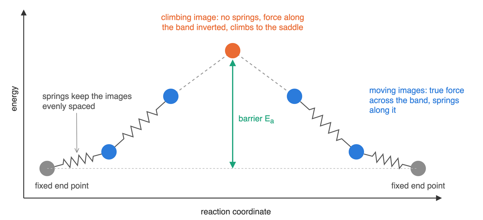
• A chain of images is placed between two relaxed minima and optimised together.

• Each moving image feels the true force perpendicular to the band and a spring force along it. The springs only keep the images evenly spaced; they do not pull the band off the minimum-energy path.

• In the climbing-image variant (CI-NEB), the highest image has no springs and the component of its true force along the band is inverted. It moves uphill along the path and downhill across it, and converges on the saddle [3]. The barrier is then read from that image, not interpolated between images.

• Cost: images × optimiser steps force calls. Every image is an independent energy and force evaluation, which suits a GPU model.

The case: Li in olivine LiFePO4

Olivine LiFePO4 is a common Li-ion cathode [1]. Li moves through one-dimensional channels along [010]; hops between channels cost more than 2.5 eV [2]. Atomistic simulations predicted a curved path between neighbouring Li sites [14], and neutron diffraction later imaged it [15]. The system is well studied with DFT, so it is a fair test for a universal MLIP.

• Cell and positions: the X-ray structure (Pnma, a = 10.332 Å, b = 6.010 Å, c = 4.692 Å) [5], from the Crystallography Open Database (entry 2100916). pymatgen expands the six symmetry-distinct sites into the 28-atom cell.

• Supercell 1×2×2 (112 atoms, 10.3 × 12.0 × 9.4 Å), the same size as a published GGA+U study [22]. Periodic copies of the vacancy are at least 9.4 Å apart.

• One Li at the origin is removed (111 atoms). The neighbouring Li along b, 3.005 Å away, hops into the vacancy.

• Both end points have the same atom order, so the band is a simple interpolation between them.

structures.py

"""Olivine LiFePO4 supercell with one Li vacancy and the two end points of a Li hop along [010]."""

from __future__ import annotations

import numpy as np
from ase import Atoms
from pymatgen.core import Lattice, Structure
from pymatgen.io.ase import AseAtomsAdaptor

# Pnma cell and sites of LiFePO4 from X-ray diffraction (Streltsov et al., 1993; COD 2100916).
CELL = (10.332, 6.010, 4.692)
SITES = [
    ("Li", (0.0, 0.0, 0.0)),
    ("Fe", (0.28222, 0.25, 0.97472)),
    ("P", (0.09486, 0.25, 0.41820)),
    ("O", (0.09678, 0.25, 0.7428)),
    ("O", (0.45710, 0.25, 0.2060)),
    ("O", (0.16558, 0.04646, 0.2848)),
]
SUPERCELL = (1, 2, 2)


def unit_cell() -> Atoms:
    species, coords = zip(*SITES)
    s = Structure.from_spacegroup("Pnma", Lattice.orthorhombic(*CELL), species, coords)
    return AseAtomsAdaptor.get_atoms(s)


def end_points(supercell: tuple[int, int, int] = SUPERCELL) -> tuple[Atoms, Atoms, int]:
    """Remove the Li at the origin; the neighbouring Li along b hops into that vacancy.

    Returns the initial and final images (same atom order) and the index of the hopping Li.
    """
    atoms = unit_cell().repeat(supercell)
    atoms.wrap()
    li = [a.index for a in atoms if a.symbol == "Li"]
    vacancy = min(li, key=lambda i: np.linalg.norm(atoms.positions[i]))
    target = atoms.positions[vacancy] + [0, CELL[1] / 2, 0]
    hopper = min(li, key=lambda i: np.linalg.norm(atoms.positions[i] - target))
    site = atoms.positions[vacancy].copy()
    del atoms[vacancy]
    hopper -= hopper > vacancy
    final = atoms.copy()
    final.positions[hopper] = site
    return atoms, final, hopper

Bond lengths of the built cell (Li–O 2.09 to 2.19 Å, Fe–O 2.06 to 2.25 Å, P–O 1.52 to 1.56 Å) match the experimental octahedra and tetrahedra.

Models

Model	Checkpoint	Training data	Reference level
MACE-MP-0b	mace-mp-0b small	MPtrj [6]	PBE and PBE+U
Orb-v3	orb-v3-conservative-inf-omat	OMat24 [7]	PBE and PBE+U
TensorNet	TensorNet-PES-MatPES-PBE-2025.2	MatPES [8]	PBE, no U

Architectures: MACE-MP-0 [9], Orb-v3 [10], TensorNet [11].

models.py

"""Three universal MLIPs as ASE calculators, all in float64."""

from __future__ import annotations

import torch

torch.set_default_dtype(torch.float64)

MODELS = {
    "MACE-MP-0b": "mace-mp-0b small (MPtrj, PBE and PBE+U)",
    "Orb-v3": "orb-v3-conservative-inf-omat (OMat24, PBE and PBE+U)",
    "TensorNet": "TensorNet-PES-MatPES-PBE-2025.2 (MatPES, PBE)",
}
MACE_MODEL = "small-0b"
MATGL_MODEL = "TensorNet-PES-MatPES-PBE-2025.2"


def device() -> str:
    return "cuda" if torch.cuda.is_available() else "cpu"


def mace():
    from mace.calculators import mace_mp

    return mace_mp(model=MACE_MODEL, device=device(), default_dtype="float64")


def orb():
    """orb-models 0.5.x API: 0.6 and later need Python 3.12, the LUMI module has 3.11."""
    from orb_models.forcefield import pretrained
    from orb_models.forcefield.calculator import ORBCalculator

    model = pretrained.orb_v3_conservative_inf_omat(device=device(), precision="float64", compile=False)
    return ORBCalculator(model, device=device())


def tensornet():
    import matgl
    from matgl.ext.ase import PESCalculator

    matgl.set_default_dtype("float", 64)
    potential = matgl.load_model(MATGL_MODEL).to(device=device(), dtype=torch.float64)
    return PESCalculator(potential, stress_unit="eV/A3")


LOADERS = {"MACE-MP-0b": mace, "Orb-v3": orb, "TensorNet": tensornet}


def load(name: str):
    """Return an ASE calculator that counts its own calculate() calls in `.calls`."""
    calc = LOADERS[name]()
    calc.calls = 0
    calculate = calc.calculate

    def counted(*args, **kwargs):
        calc.calls += 1
        return calculate(*args, **kwargs)

    calc.calculate = counted
    return calc


def versions() -> dict:
    from importlib.metadata import version

    pkgs = ("torch", "ase", "pymatgen", "mace-torch", "orb-models", "matgl")
    out = {p: version(p) for p in pkgs}
    out["gpu"] = torch.cuda.get_device_name(0) if torch.cuda.is_available() else None
    out["float"] = str(torch.get_default_dtype()).removeprefix("torch.")
    return out

On LUMI, torch 2.7.1+rocm6.2.4 fails in float32 det and prod kernels (CUDA driver error: 209), so every model runs in float64. The module has Python 3.11, so orb-models is 0.5.5 (0.6 and later need Python 3.12).

NEB set-up

• Relax both end points at fixed cell with FIRE [12] to fmax 0.05 eV/Å.

• Seven moving images, first guess from IDPP [13], which avoids atoms coming too close in a straight-line guess.

• CI-NEB in ASE [4] from the start, spring constant 0.1 eV/Ų (ASE default), FIRE to fmax 0.05 eV/Å, at most 1000 steps.

• Barrier: highest image energy minus the initial energy. Force calls: model evaluations counted in the calculator. Wall time: the NEB optimisation only.

neb.py

def run(name: str, images: int = 7, fmax: float = 0.05, optimiser: str = "FIRE",
        steps: int = 1000) -> dict:
    opt = OPTIMISERS[optimiser]
    calc = models.load(name)
    initial, final, hopper = structures.end_points()

    start = time.perf_counter()
    relaxed = []
    for atoms in (initial, final):
        atoms.calc = calc
        relaxed.append(bool(opt(atoms, logfile=None).run(fmax=fmax, steps=steps)))
        freeze(atoms)
    relax = {"converged": relaxed, "force_calls": calc.calls,
             "wall_s": round(time.perf_counter() - start, 2)}

    band = [initial] + [initial.copy() for _ in range(images)] + [final]
    for atoms in band[1:-1]:
        atoms.calc = ImageCalculator(calc)
    neb = NEB(band, climb=True)
    neb.interpolate(method="idpp", mic=True)
    calc.calls = 0
    start = time.perf_counter()
    optimizer = opt(neb, logfile=None)
    converged = bool(optimizer.run(fmax=fmax, steps=steps))
    neb_run = {"converged": converged, "steps": optimizer.nsteps, "force_calls": calc.calls,
               "wall_s": round(time.perf_counter() - start, 2)}
    for atoms in band[1:-1]:
        freeze(atoms)

    tools = NEBTools(band)
    barrier, delta = tools.get_barrier(fit=False)
    fit = tools.get_fit()
    e0 = band[0].get_potential_energy()
    result = {
        "model": name, "description": models.MODELS[name], "atoms": len(initial),
        "images": images, "fmax": fmax, "optimiser": optimiser,
        "barrier_eV": round(float(barrier), 4), "reaction_energy_eV": round(float(delta), 4),
        "hop_distance_A": round(float(fit.path[-1]), 4),
        "relax": relax, "neb": neb_run,
        "path_A": [round(float(x), 4) for x in fit.path],
        "energies_eV": [round(float(a.get_potential_energy() - e0), 5) for a in band],
        "fit_path_A": [round(float(x), 4) for x in fit.fit_path],
        "fit_energies_eV": [round(float(x), 5) for x in fit.fit_energies],
        "li_offset_xz_A": lateral_offset(band, hopper),
        "hopper": hopper,
    }
    RESULTS.mkdir(exist_ok=True)
    stem = name.lower().replace("-", "_")
    (RESULTS / f"{stem}.json").write_text(json.dumps(result, indent=2))
    write(RESULTS / f"{stem}_band.extxyz", band)
    return result

One model is loaded once and shared by all images. If the images share one ASE calculator directly (allow_shared_calculator=True), its cache only holds the last image, and ASE evaluates every image again each time the optimiser asks the band for forces: about three times per step. A thin per-image wrapper keeps a cache for each image:

neb.py: ImageCalculator

class ImageCalculator(Calculator):
    """Per-image view of one shared model, so each image caches its own results.

    With one calculator shared by all images, ASE re-evaluates every image each time
    the optimiser asks the band for forces (about three times per step).
    """

    implemented_properties = ["energy", "forces"]

    def __init__(self, model):
        super().__init__()
        self.model = model

    def calculate(self, atoms=None, properties=("energy",), system_changes=all_changes):
        super().calculate(atoms, properties, system_changes)
        copy = self.atoms.copy()
        copy.calc = self.model
        self.results = {"energy": copy.get_potential_energy(), "forces": copy.get_forces()}

Run on LUMI

On a login node (compute nodes have no internet), in a copy of this repository at <SCRATCH>/mlip-neb:

module purge && module use /appl/local/csc/modulefiles/ && module load pytorch
python -m venv --system-site-packages .venv && source .venv/bin/activate
pip install -r examples/neb/requirements.txt
for m in MACE-MP-0b Orb-v3 TensorNet; do
    HF_HOME=$PWD/hf-home python examples/neb/cli.py prefetch --model $m
done
sbatch --account=<PROJECT> scripts/lumi-neb.sbatch

The job runs each model in its own process, then draws the figures, and ends with:

MACE-MP-0b: barrier 0.263 eV, NEB 343 calls, 12.01 s, converged True
Orb-v3: barrier 0.317 eV, NEB 329 calls, 19.37 s, converged True
TensorNet: barrier 0.143 eV, NEB 252 calls, 7.33 s, converged True
== done ..., failed: none

lumi-neb.sbatch

export PYTHONNOUSERSITE=1
export HF_HOME="$root/hf-home" HF_HUB_OFFLINE=1
export MIOPEN_USER_DB_PATH="/tmp/$USER-miopen-$SLURM_JOB_ID"
export MIOPEN_CUSTOM_CACHE_DIR="$MIOPEN_USER_DB_PATH"
export HIP_FORCE_DEV_KERNARG=1
export MPLCONFIGDIR="/tmp/$USER-mpl-$SLURM_JOB_ID"
export OMP_NUM_THREADS="$SLURM_CPUS_PER_TASK"
mkdir -p "$MIOPEN_USER_DB_PATH" "$MPLCONFIGDIR"
trap 'rm -rf "$MIOPEN_USER_DB_PATH" "$MPLCONFIGDIR"' EXIT

cd "$root/examples/neb"
run() { srun --ntasks=1 --gpus=1 --cpu-bind=cores python cli.py "$@"; }
failed=()
run versions || failed+=(versions)
for model in MACE-MP-0b Orb-v3 TensorNet; do
    echo "== $model $(date +%T)"
    run run --model "$model" || failed+=("$model")
done
run figures || failed+=(figures)
echo "== done $(date +%T), failed: ${failed[*]:-none}"

cli.py

def main() -> None:
    parser = argparse.ArgumentParser(description=__doc__)
    parser.add_argument("step", choices=STEPS)
    parser.add_argument("--model", choices=list(models.MODELS), help="model for run (default: all)")
    parser.add_argument("--images", type=int, default=7, help="moving images between end points")
    parser.add_argument("--fmax", type=float, default=0.05, help="force tolerance (eV/Å)")
    parser.add_argument("--optimiser", choices=["FIRE", "BFGS"], default="FIRE")
    args = parser.parse_args()
    names = [args.model] if args.model else list(models.MODELS)

    if args.step == "prefetch":
        for name in names:
            models.load(name)
            print("cached", name)
    elif args.step == "versions":
        import neb

        neb.RESULTS.mkdir(exist_ok=True)
        text = json.dumps(models.versions(), indent=2)
        (neb.RESULTS / "versions.json").write_text(text)
        print(text)
    elif args.step == "run":
        import neb

        for name in names:
            r = neb.run(name, images=args.images, fmax=args.fmax, optimiser=args.optimiser)
            print(f"{name}: barrier {r['barrier_eV']:.3f} eV, NEB {r['neb']['force_calls']} calls, "
                  f"{r['neb']['wall_s']} s, converged {r['neb']['converged']}")
    else:
        import figures

        figures.main()


if __name__ == "__main__":
    main()

To vary one setting inside a GPU allocation, from examples/neb (this overwrites that model’s files in results/):

python cli.py run --model TensorNet --optimiser BFGS
python cli.py run --model MACE-MP-0b --images 5 --fmax 0.03

Results

Conditions: one AMD MI250X GCD, float64, one run, 111 atoms, 7 moving images, torch 2.7.1+rocm6.2.4, ase 3.29.0, pymatgen 2026.9.24, mace-torch 0.3.16, orb-models 0.5.5, matgl 4.0.3.

	MACE-MP-0b	Orb-v3	TensorNet
barrier Ea	0.263 eV	0.317 eV	0.143 eV
end-point energy difference	0.000 eV	0.000 eV	0.000 eV
NEB steps	48	46	35
NEB force calls	343	329	252
NEB wall time	12.0 s	19.4 s	7.3 s
time per force call	35 ms	59 ms	29 ms
end-point relaxation (2 structures)	74 calls, 16.9 s	90 calls, 19.3 s	78 calls, 3.0 s
path length of the hopping Li	3.35 Å	3.26 Å	3.24 Å
offset from straight line at saddle	0.67 Å	0.65 Å	0.64 Å

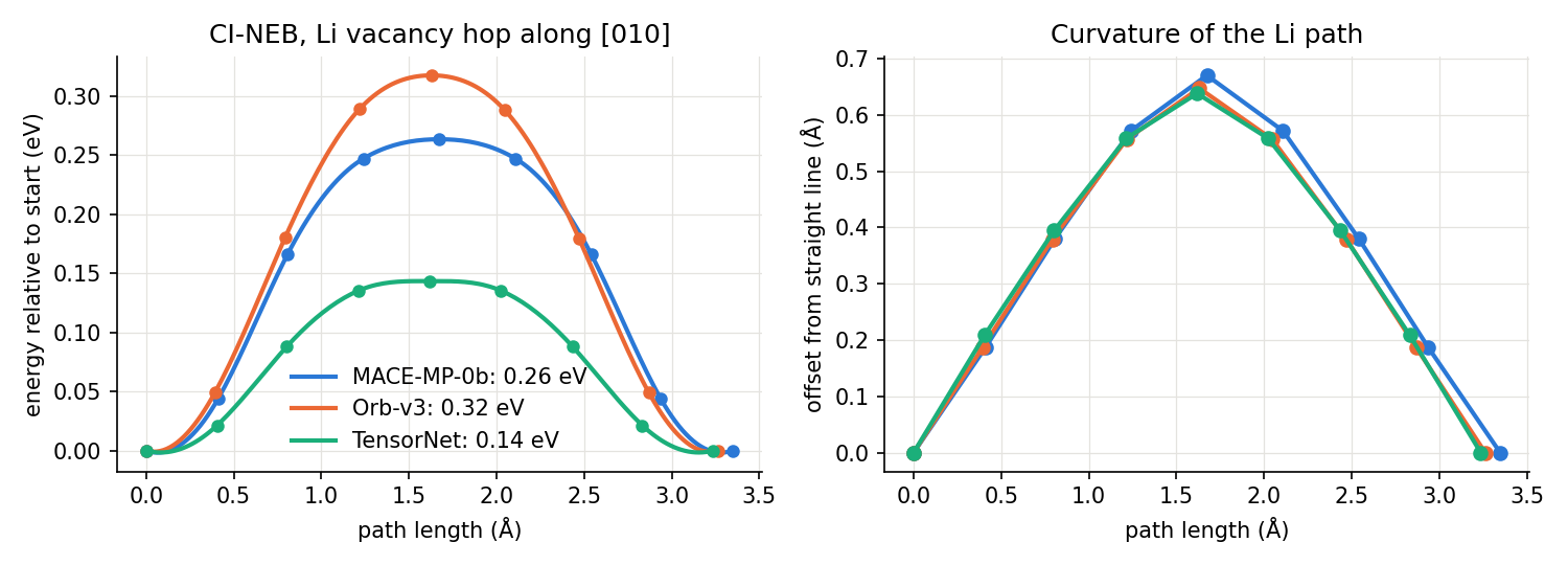
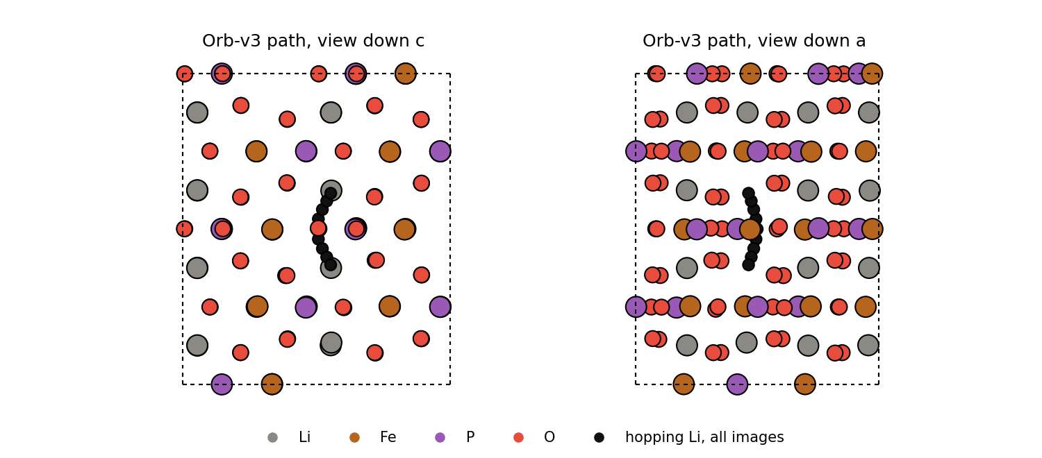
• All three runs converged, and both end points have the same energy, as the symmetry of the hop requires.

• All three find the curved path: the Li bulges 0.64 to 0.67 Å off the straight line, so it travels about 3.3 Å instead of 3.0 Å, as predicted [14] and observed [15].

• The end-point relaxation times include loading the model and GPU warm-up; use the NEB times to compare cost.

• With one shared calculator (allow_shared_calculator=True) the same job needed 1022, 980 and 749 force calls and 34.4, 56.3 and 20.6 s for the same barriers. The per-image wrapper saves about a factor of three.

Comparison with DFT and experiment

Method	Barrier
GGA (PW91), ferromagnetic, vacancy in LiFePO4 [2]	0.27 eV
GGA+U (U = 4.3 eV), vacancy, hole on an in-plane Fe [16]	0.29 eV
GGA+U, vacancy, hole on an out-of-plane Fe [16]	0.47 eV
GGA+U, charged vacancy, 1×2×2 cell [22]	0.32 eV
Classical shell-model potentials [14]	0.55 eV
Experiment, single-crystal impedance along b [24]	about 0.54 eV
Experiment, single-crystal muon spin relaxation [23]	0.14 to 0.17 eV
MACE-MP-0b, Orb-v3, TensorNet (this page)	0.26, 0.32, 0.14 eV

• MACE-MP-0b and Orb-v3 fall within 0.05 eV of the DFT vacancy barriers without a localised hole (0.27 to 0.32 eV).

• TensorNet gives about half. The missing U is not the main cause, since plain GGA gives 0.27 eV [2]; a too soft energy surface is the likely reason (next section).

• The 0.17 eV spread between models is close to a factor of 1000 in hop rate at 298 K.

• Experiments do not measure the same quantity. Macroscopic transport (about 0.5 eV and higher) includes antisite defects that block channels and polarons; muon spin relaxation probes local hops. Compare an MLIP with the DFT level it was trained on, not with experiment.

Reading the results

Softening: expect underestimates

Universal MLIPs are trained mostly on structures near equilibrium. Far from it, their energy surface is too flat (“softened”), and energies and forces of high-energy states such as saddle points come out too low [17].

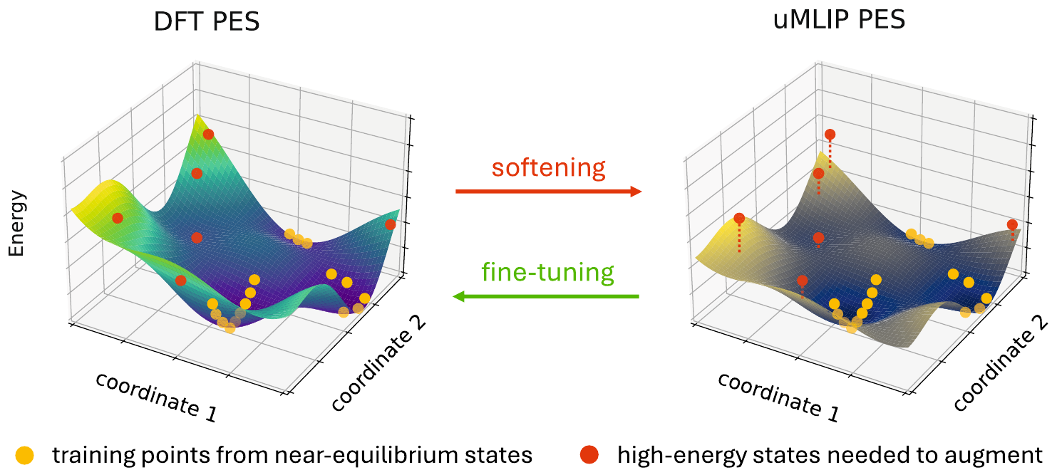
Figure: B. Deng et al., npj Comput. Mater. 11, 9 (2025), Fig. 1 [17], CC BY 4.0; caption removed.

For 470 Mg²⁺ migration paths (reference: ApproxNEB with GGA), MACE-MP-0, CHGNet and M3GNet gave barrier mean absolute errors (MAE) of 0.34, 0.39 and 0.49 eV, and all three distributions are shifted to negative errors:

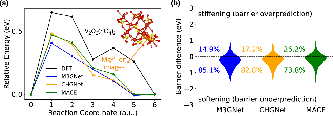
Figure: B. Deng et al., npj Comput. Mater. 11, 9 (2025), Fig. 3 [17], CC BY 4.0, unmodified.

The same work shows the error is systematic: fine-tuning CHGNet on one structure moved its force-slope from 0.86 to 0.97 of DFT, and ten structures cut the force MAE from 0.19 to 0.13 eV/Å (see A4 Train and fine-tune a potential).

How good are zero-shot barriers?

The largest solid-state test ran five universal MLIPs, unchanged, on 574 battery migration paths with GGA DFT-NEB references [18]. Their NEB had no climbing image and only three moving images, so each band maximum is a lower bound on the model’s own saddle. Its Orb-v3 is the checkpoint used on this page; its MACE-MP-0 is the large MPtrj model, not MACE-MP-0b small.

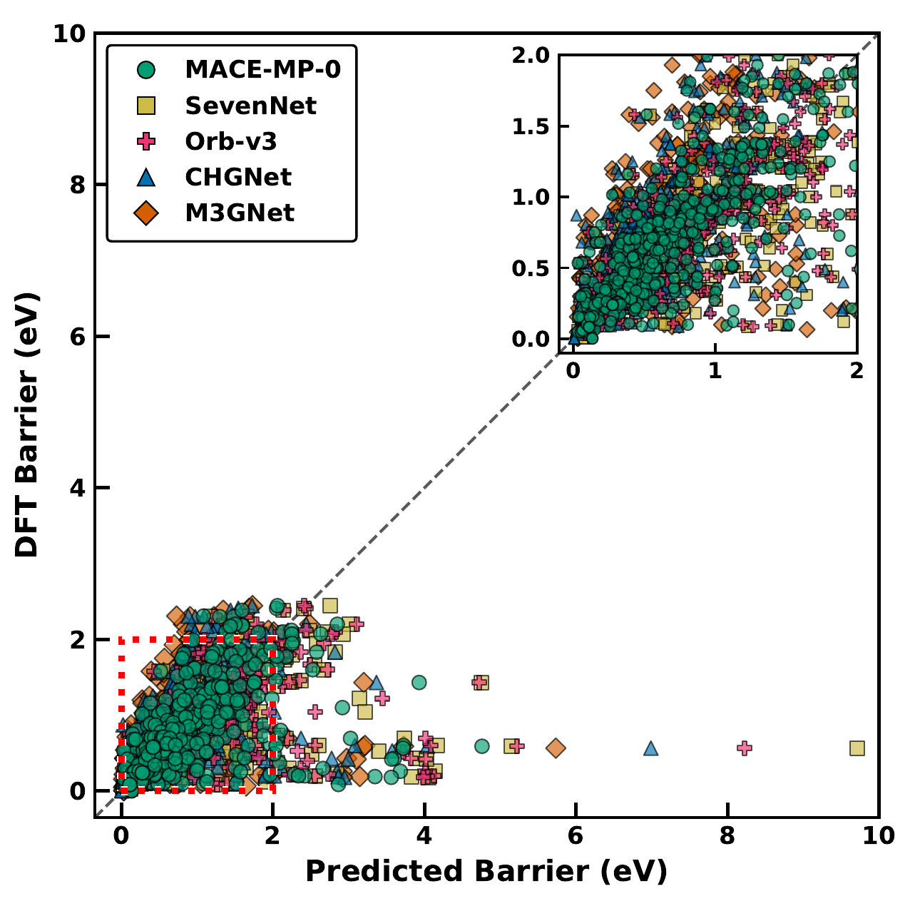
Figure: A. K. Bheemaguli, P. Xiao and G. Sai Gautam, Fig. 2 of arXiv:2512.03642 [18], CC BY 4.0, cropped to the plot.

	MACE-MP-0	Orb-v3	SevenNet	CHGNet	M3GNet
MAE, all 574 paths	0.310 eV	0.336 eV	0.344 eV	0.343 eV	0.349 eV
MAE, 17 common outliers removed	0.239 eV	0.245 eV	0.251 eV	0.275 eV	0.290 eV
MAE, each model’s outliers above 1 eV removed	0.202 eV	0.198 eV	0.203 eV	0.248 eV	0.257 eV
correct good/bad at 0.5 eV	79.4 %	84.8 %	82.9 %	73.9 %	73.5 %
underestimated paths	52 %	42 %	43 %	73 %	78 %

• An MAE of 0.2 to 0.3 eV is far too large for a quantitative rate, but good enough to sort fast from slow conductors about 80 % of the time.

• CHGNet and M3GNet underestimate most barriers; MACE, SevenNet and Orb-v3 show no clear bias on this set.

• The MLIP path is a good start: the MLIP images were better first guesses for DFT than a linear interpolation in about 66 % of cases (above 71 % for MACE-MP-0 and SevenNet).

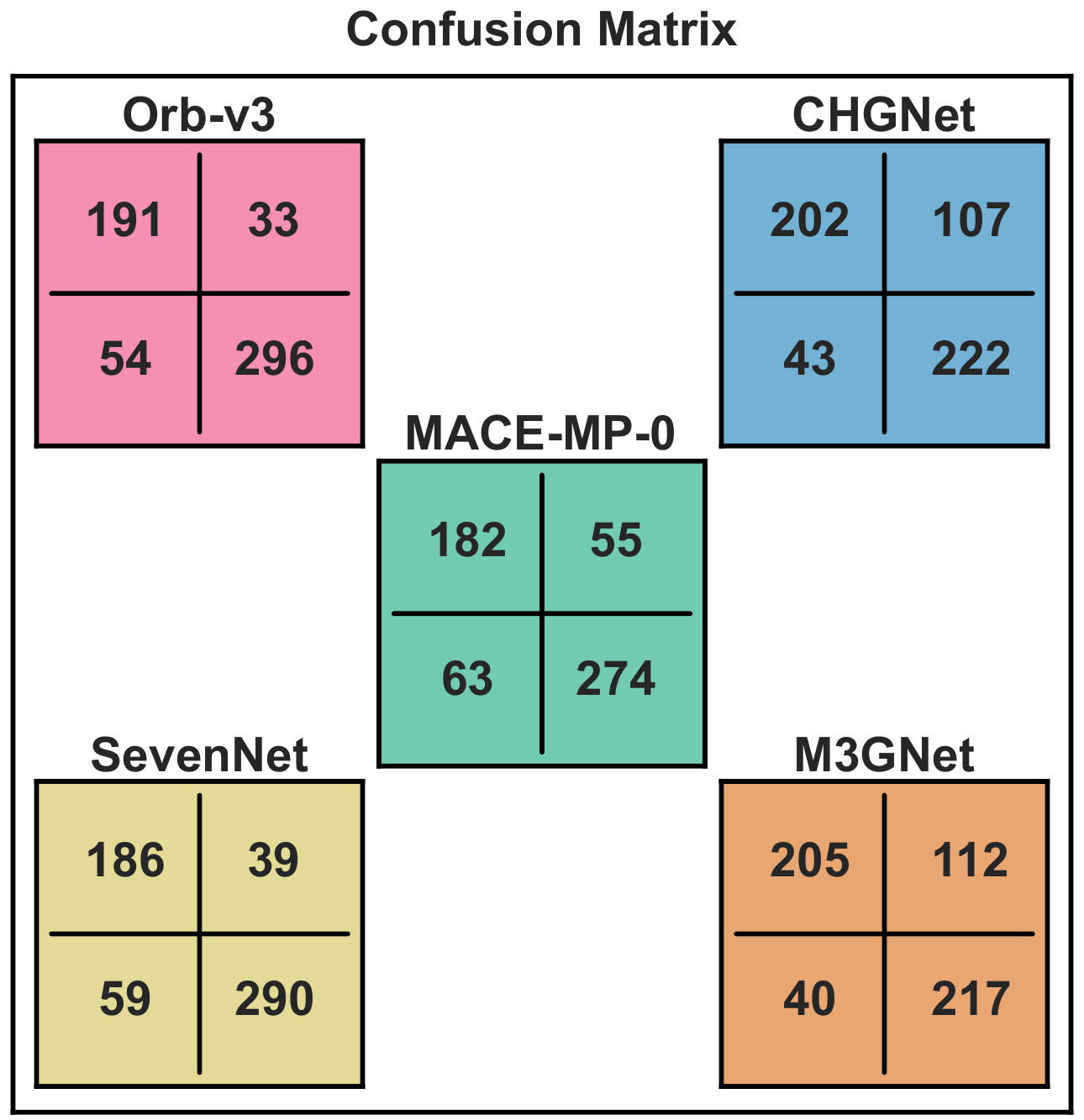
Figure: A. K. Bheemaguli, P. Xiao and G. Sai Gautam, Fig. 4 of arXiv:2512.03642 [18], CC BY 4.0, cropped to the plot.

Newer models trained on more off-equilibrium data do better. On 154 DFT-NEB ion-migration paths with a full CI-NEB workflow, barrier MAE ranged from about 0.05 eV (UMA) and 0.06 eV (MACE-MPA-0) to 0.10 to 0.17 eV for MatPES and older models, and most models still underestimated [20]. Static evaluations along the DFT paths gave similar errors, so the error comes from the energy surface, not from the NEB.

Screening, then refinement

The most reliable use of an MLIP-NEB is as a cheap first stage whose path and saddle are checked with a few DFT calculations. For 932 surface reactions (OC20NEB, RPBE), models trained only on adsorbate relaxations found transition states within 0.1 eV of DFT 91 % of the time, with a 28× speed-up [19]. The two numbers come from different model sizes; the trade-off for one model is in panel d below.

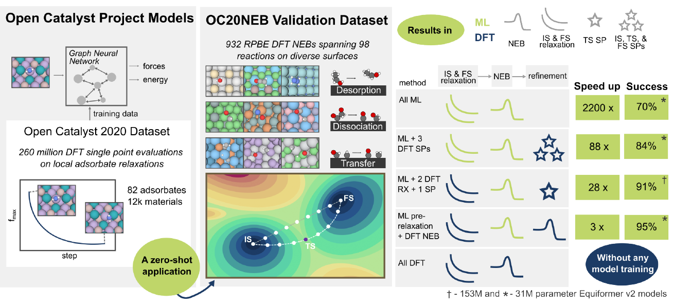
Figure: B. Wander et al., Fig. 1 of arXiv:2405.02078 [19], CC BY 4.0, cropped to the figure.

Protocol (EquiformerV2, 31M)	Speed-up	Success within 0.1 eV
all ML	2200×	70 %
ML, then 3 DFT single points	88×	84 %
ML, then 2 DFT relaxations and 1 DFT single point	28×	88 %
ML pre-relaxation, then DFT NEB	3×	DFT level

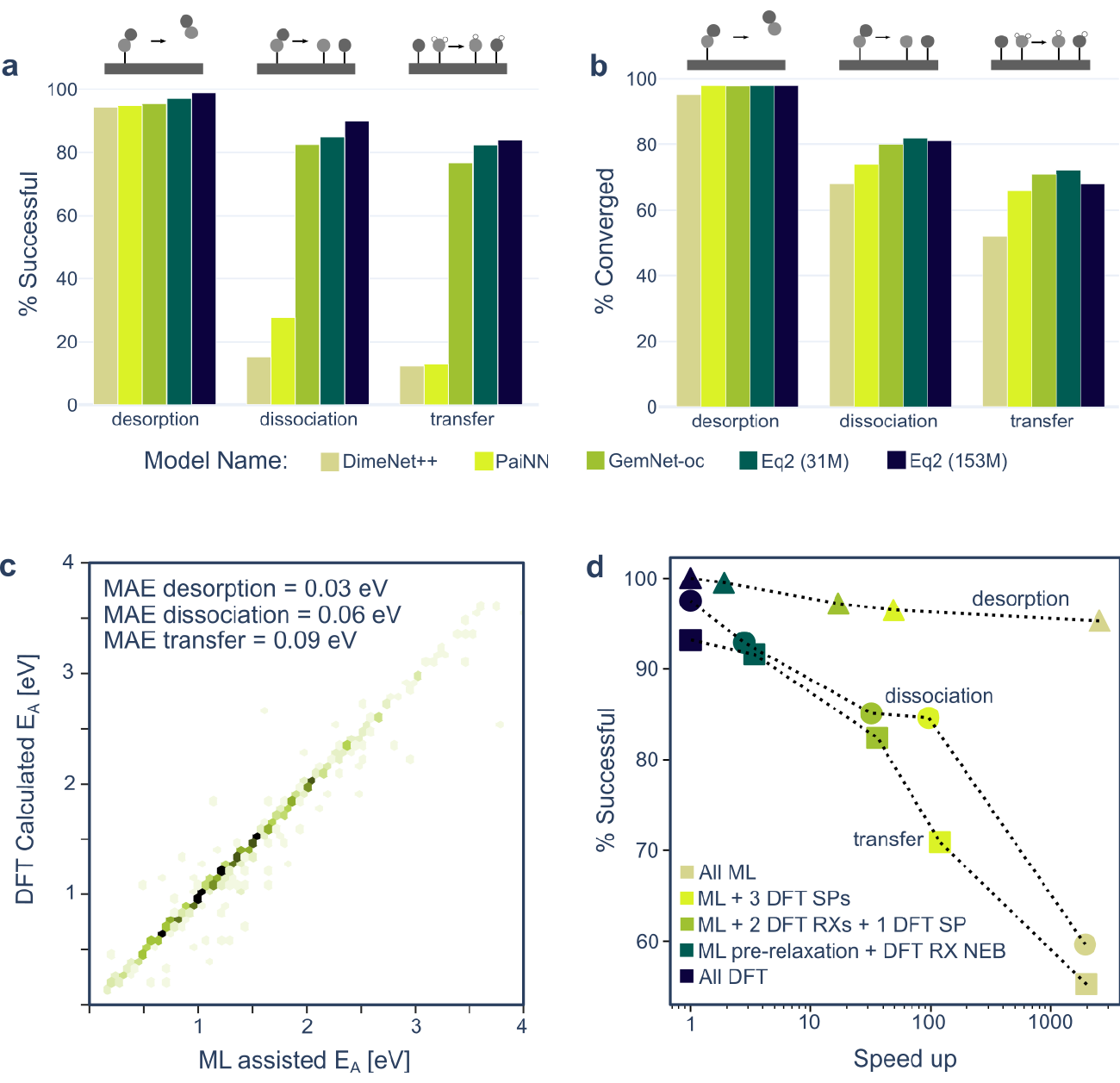
Figure: B. Wander et al., Fig. 2 of arXiv:2405.02078 [19], CC BY 4.0, cropped to the figure.

• A full reaction network (CO hydrogenation on Rh(111), about 19 000 NEBs) took 12 GPU days, against an estimated 52 GPU years with DFT.

• ML pre-optimised bands sometimes found lower transition states than DFT alone (7 % of transfers), since cheap sampling explores more paths.

• For organic molecules, MLIP path searches followed by DFT saddle refinement reached 96.6 % success (MACE-OMol25) with 3.8 DFT gradients per reaction, 94 to 96 % fewer than DFT alone [21].

• Uncertainty-aware NEB, which weights forces by the model’s force covariance, is an early research direction [25].

For LiFePO4 this means: take the MLIP path and saddle geometry, then run a few DFT (+U) single points or a short DFT CI-NEB started from the MLIP band.

Magnetism, charge and PBE+U

• Fe²⁺ in LiFePO4 carries a magnetic moment. These MLIPs take no spins or charges as input: they were trained mostly on spin-polarised DFT, but predict one energy surface without a magnetic state.

• Removing a neutral Li leaves a hole on a nearby Fe (Fe³⁺). The models cannot place this polaron, so the result is closest to a DFT calculation with a delocalised hole.

• Where the hole sits changes the DFT barrier by almost 0.2 eV [16], more than the spread between MACE-MP-0b and Orb-v3. Polaron effects need DFT+U or hybrid DFT.

• MPtrj and OMat24 mix PBE and PBE+U labels; MatPES is PBE only. Know which reference a model reproduces before comparing it with a DFT+U number.

Keypoints

• CI-NEB with a universal MLIP gives the curved Li path in LiFePO4 and a barrier in seconds on one GPU; barriers differ by a factor of two between models (0.14 to 0.32 eV).

• Zero-shot MLIP barriers have mean errors of 0.05 to 0.5 eV and tend to be too low (softening): good for ranking and paths, not for rates.

• Use MLIP-NEB to screen and to start DFT; refine the saddle with DFT, especially where magnetism or polarons matter.

References

1. A. K. Padhi et al., J. Electrochem. Soc. 144, 1188 (1997). doi:10.1149/1.1837571

2. D. Morgan, A. Van der Ven and G. Ceder, Electrochem. Solid-State Lett. 7, A30 (2004). doi:10.1149/1.1633511

3. G. Henkelman, B. P. Uberuaga and H. Jónsson, J. Chem. Phys. 113, 9901 (2000). doi:10.1063/1.1329672

4. A. Hjorth Larsen et al., ASE, J. Phys.: Condens. Matter 29, 273002 (2017). doi:10.1088/1361-648X/aa680e

5. V. A. Streltsov et al., Acta Cryst. B 49, 147 (1993). doi:10.1107/S0108768192004701

6. B. Deng et al., CHGNet and MPtrj, Nat. Mach. Intell. 5, 1031 (2023). doi:10.1038/s42256-023-00716-3

7. L. Barroso-Luque et al., OMat24. arXiv:2410.12771

8. A. D. Kaplan et al., MatPES. arXiv:2503.04070

9. I. Batatia et al., MACE-MP-0. arXiv:2401.00096

10. B. Rhodes et al., Orb-v3. arXiv:2504.06231

11. G. Simeon and G. De Fabritiis, TensorNet. arXiv:2306.06482

12. E. Bitzek et al., FIRE, Phys. Rev. Lett. 97, 170201 (2006). doi:10.1103/PhysRevLett.97.170201

13. S. Smidstrup et al., IDPP, J. Chem. Phys. 140, 214106 (2014). doi:10.1063/1.4878664

14. M. S. Islam et al., Chem. Mater. 17, 5085 (2005). doi:10.1021/cm050999v

15. S. Nishimura et al., Nat. Mater. 7, 707 (2008). doi:10.1038/nmat2251

16. G. K. P. Dathar et al., Chem. Mater. 23, 4032 (2011). doi:10.1021/cm201604g

17. B. Deng et al., Systematic softening in universal machine learning interatomic potentials, npj Comput. Mater. 11, 9 (2025). doi:10.1038/s41524-024-01500-6

18. A. K. Bheemaguli, P. Xiao and G. Sai Gautam, Evaluation of foundational machine learned interatomic potentials for migration barrier predictions, Digital Discovery 5, 1809 (2026). doi:10.1039/D5DD00534E; arXiv:2512.03642; code and data, Zenodo

19. B. Wander et al., CatTSunami, ACS Catal. 15, 5283 (2025). doi:10.1021/acscatal.4c04272; arXiv:2405.02078

20. K. Amirian et al., FPBench. arXiv:2609.05714; code

21. J. Marks, J. Vandezande and J. Gomes, automated transition-state searches with MLIPs. arXiv:2604.00405

22. K. Hoang and M. Johannes, Chem. Mater. 23, 3003 (2011). doi:10.1021/cm200725j; arXiv:1105.3492

23. O. K. Forslund et al., single-crystal muon spin relaxation of LiFePO4. arXiv:2111.11941

24. J. Li, W. Yao, S. Martin and D. Vaknin, Solid State Ionics 179, 2016 (2008). doi:10.1016/j.ssi.2008.06.028

25. Y. Yu and Y. Wang, uncertainty-aware NEB and dimer methods. arXiv:2605.24401